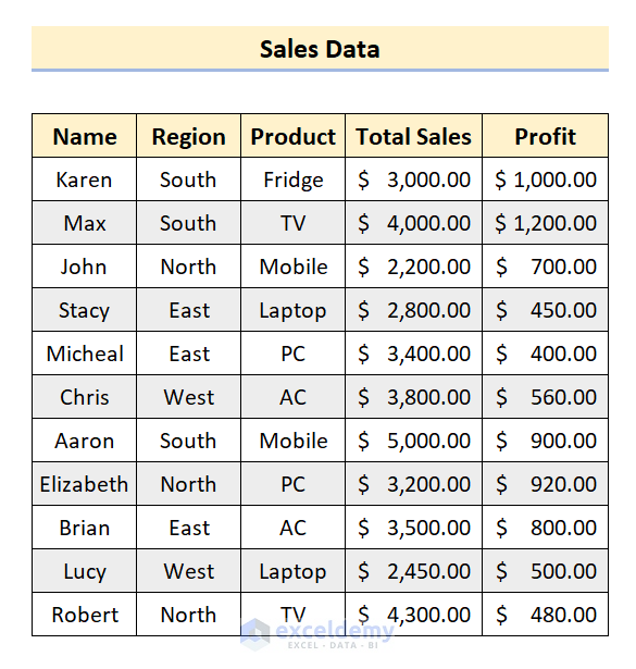
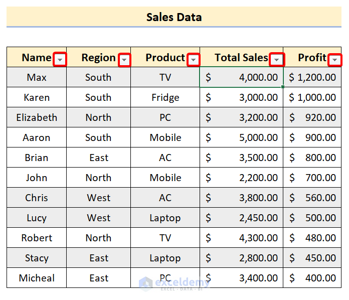
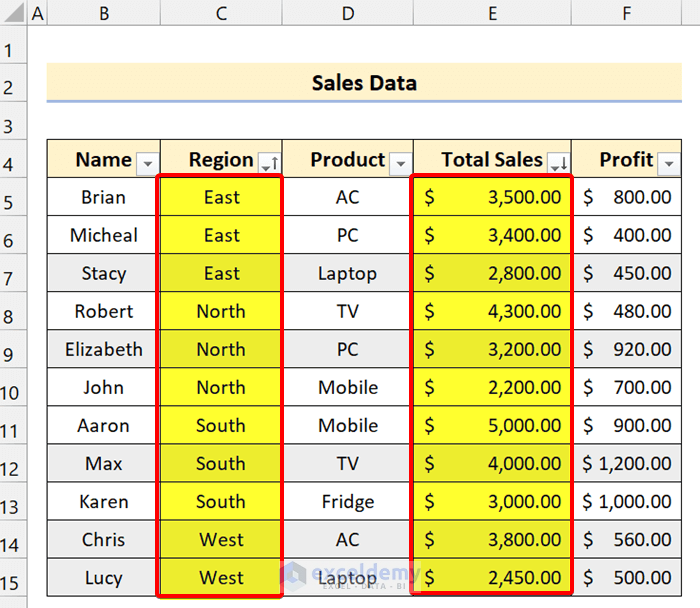
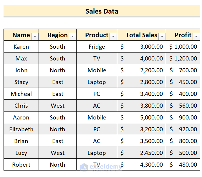
This is the sample dataset:
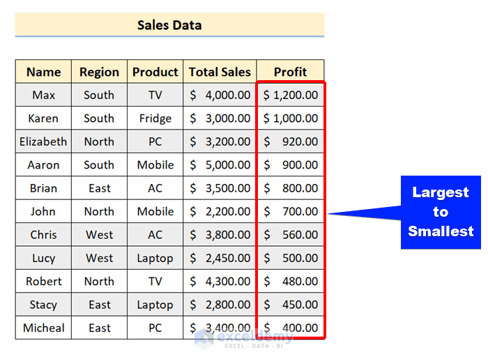
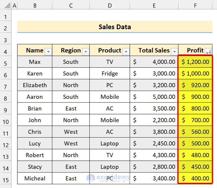
After sorting data based on Profit, in descending order:
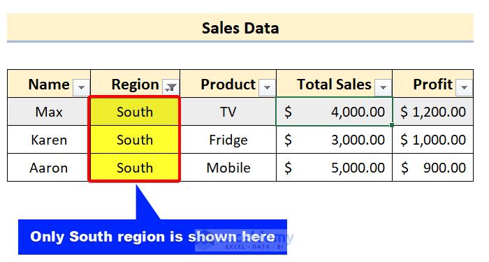
Filter the dataset based on “South”:
How to Enable Sort And Filter in Excel
- Click any cell in the dataset.
- Go to the Data tab.
- In Sort & Filter, click Filter.
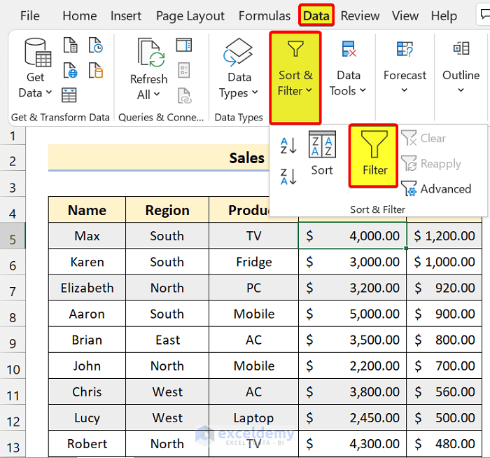
You will see the dropdown beside every column header.
Types of Sort in Excel
1. Sort in Alphabetical Order
Choose A to Z or Z to A.
Steps
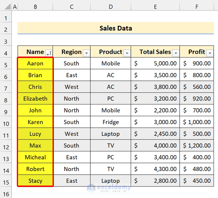
- Click the dropdown menu beside “Name”.
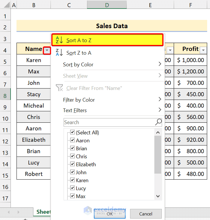
- Click Sort A to Z to sort the Name column in ascending order.
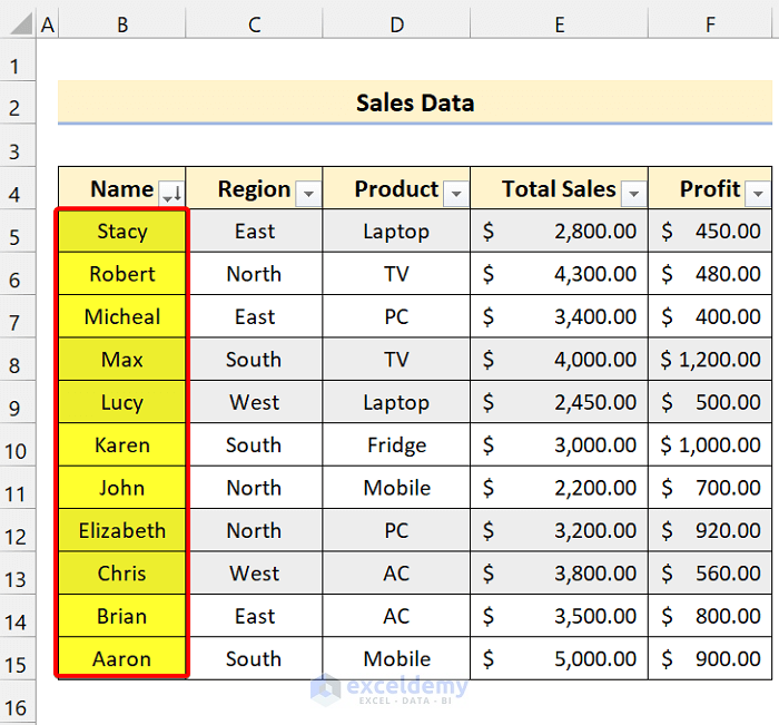
- If you click Sort Z to A, data will be sorted in descending order.
Read More: How to Perform Random Sort in Excel
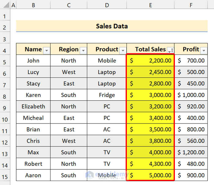
2. Sort by Smallest to Largest in Excel
If you have numerical data, sort it from smallest to largest.
Steps
- Click the dropdown menu beside the Total Sales column.
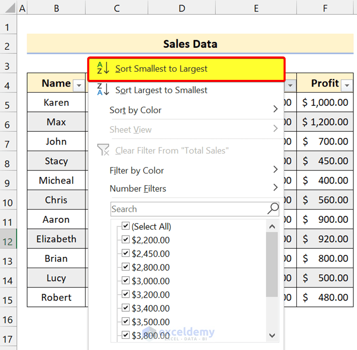
- Click Sort Smallest to Largest.
3. Sort by Largest to Smallest
Sort data in the Profit column.
Steps
- Click the dropdown menu beside the Profit column.
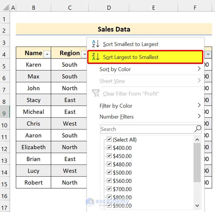
- Click Sort Largest to Smallest.
Read More: How to Sort Excel Tabs
4. Multi-level Sort in Excel
- Sort data based on Region (A to Z).
- Sort it again based on Total Sales (Largest to Smallest).
Steps
- Click the dropdown menu beside “Region”.
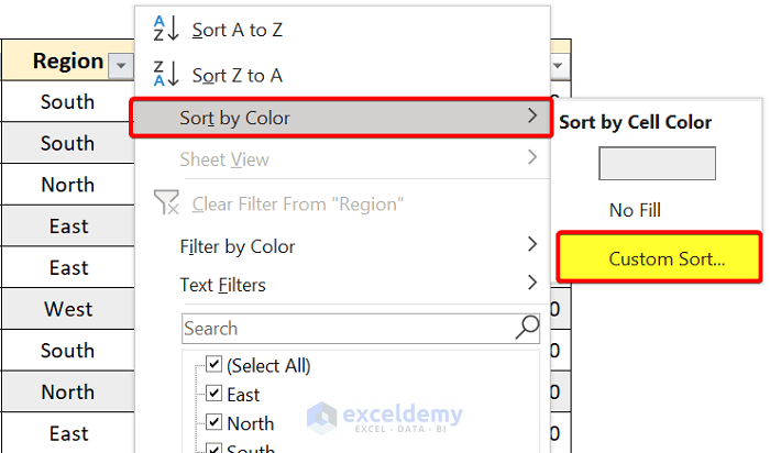
- Select Sort by Color.
- Click Custom Sort.
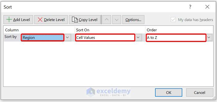
- Select Region in Sort by.
- Select Cell values and A to Z.
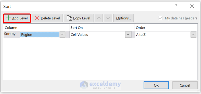
- Click Add Level.
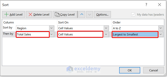
- Select Total Sales in Then by.
- Select Cell values and Largest to Smallest.
- Click OK.
5. SORT Function
To sort data based on the Product column in Descending order:
Steps
- Enter the following formula in H5:
=SORT(B5:F15,3,-1)
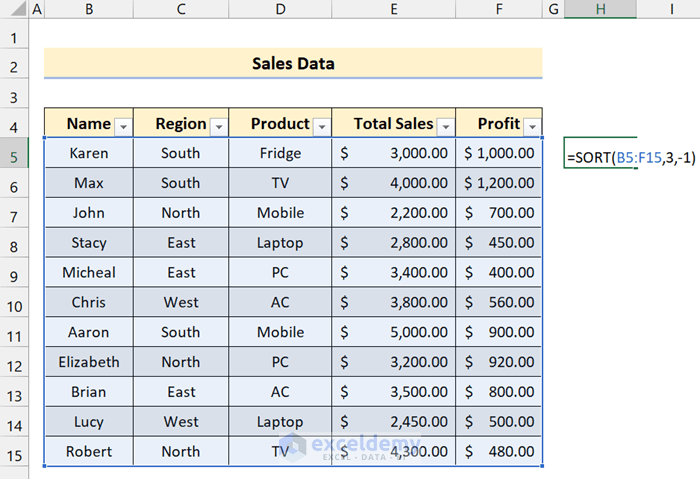
- Press Enter.

Read More: Advantages of Sorting Data in Excel
Types of Filter in Excel
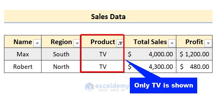
1. Regular Filter
You can filter data based on any values.
Filter the dataset based on “TV”:
Steps
- Click the dropdown menu beside Product.
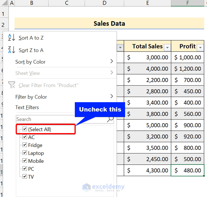
- Uncheck Select All.
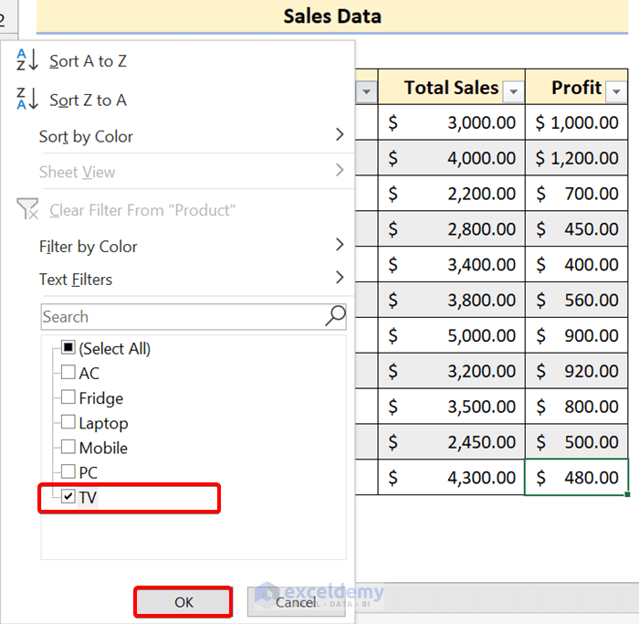
- Check“TV” and click OK.
2. Text Filters / Number Filters in Excel
Filter text with Text Filters. Excel automatically shows Number Filters in columns containing numeric values.
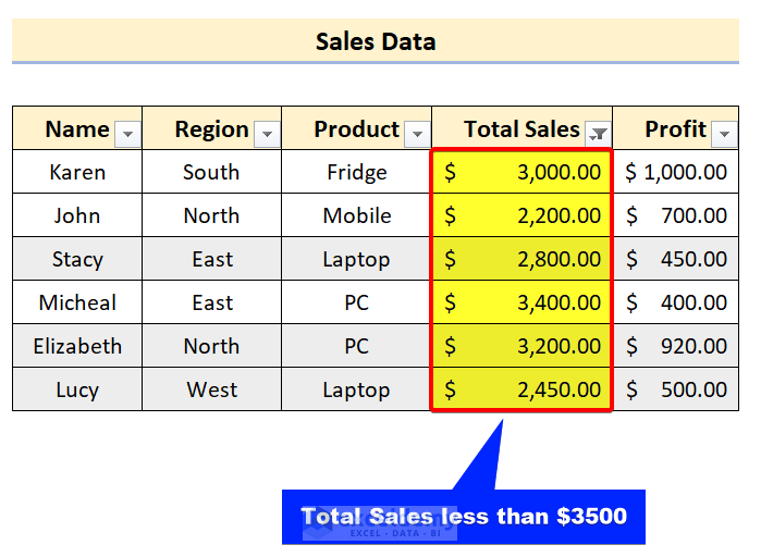
Filter the dataset based on the Total Sales less than $3500.
Steps
- Click the dropdown menu beside Total Sales.
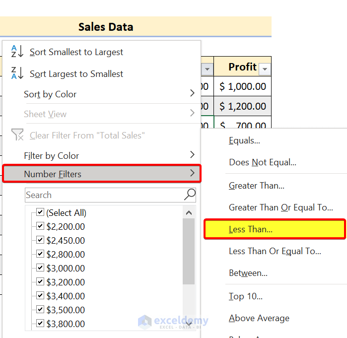
- Select Number Filters and click Less Than.
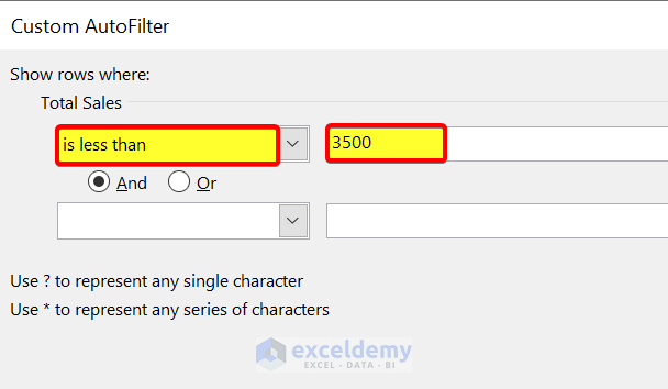
- Enter $3500.
- Click OK.
Read More: How to Perform Custom Sort in Excel
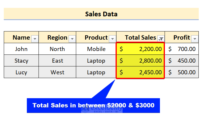
3. Custom Filter
To filter data based on the Total Sales greater than $2000 but less than $3000:
Steps
- Click the dropdown menu beside Total Sales.
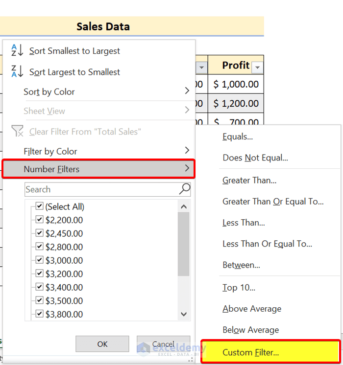
- Select Number Filters and click Custom Filter.
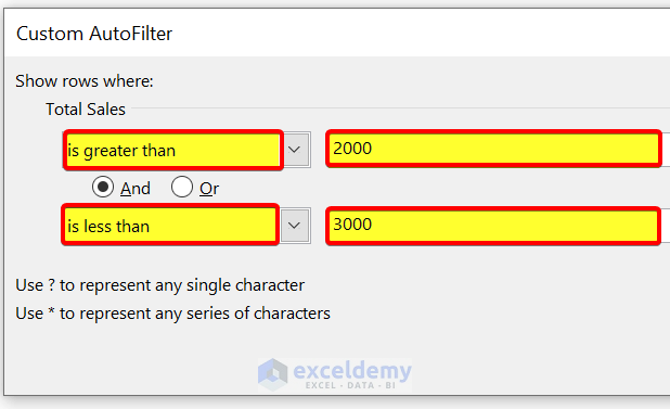
- Enter the values.
- Select And and click OK.
Read More: Advanced Sorting in Excel
How to Undo Sort and Filter in Excel
1. Undo Sort:
- Click Undo or press Ctrl+Z.
Or:
- Create a temporary column.
2. Undo Filter
- Click the dropdown menu to which you applied filtering.
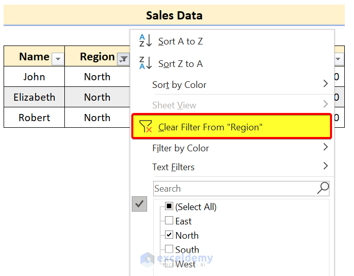
- Click Clear Filter From “Region” (column name can be different based on your filtering).
To remove the dropdown menu:
- Click any cell in your dataset.
- Go to the Data tab.
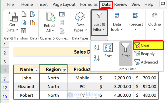
- In Sort & Filter, click Clear.
Read More: Difference Between Sort and Filter in Excel
Download Practice Workbook
Download the practice workbook.
Related Articles
<< Go Back to Sort in Excel | Learn Excel
Get FREE Advanced Excel Exercises with Solutions!
