How to Do Advanced Sorting in Excel (9 Suitable Examples)

In this article, we will demonstrate several effective techniques for Advanced Sorting in Excel:

Sorting from top to bottom.
Sorting from left to right.
Multi-level sorting.
Case-sensitive sorting.
Sorting based on cell color and font color.
Sorting using conditional formatting.
Using a custom list to sort.
Using the SORT and SORTBY functions

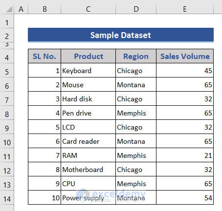
We’ll use the dataset below to illustrate our methods.

Method 1 – Sorting from Top to Bottom

Steps:

Select a column to sort, for example Column C.
Go to the Data tab and click the icon indicated in the image below.

A Sort Warning box appears.

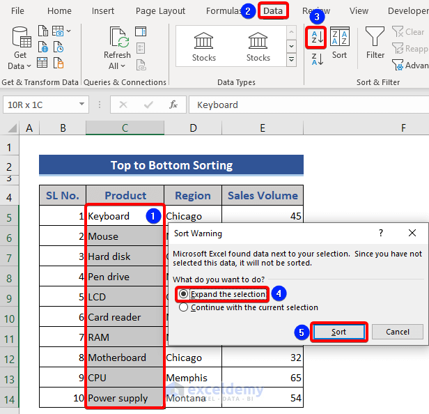
Click on Expand the selection and click the Sort button.

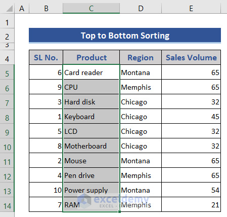
Column C is sorted in ascending alphabetical order, along with the rest of the dataset.

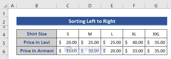
Method 2 – Sorting from Left to Right

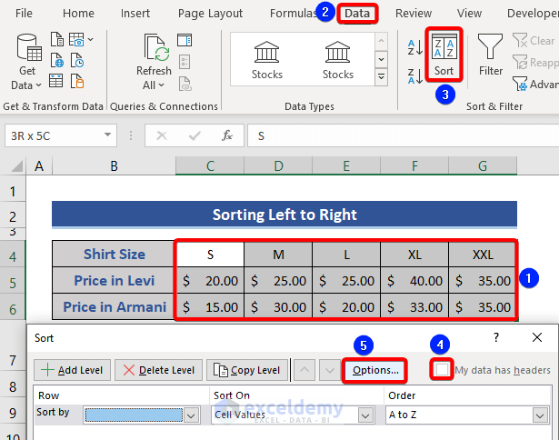
Prices of different types of shirt sizes are given in the dataset below. Let’s sort these shirt sizes in ascending alphabetical order from left to right.

Steps:

Select Rows 4 to 6.
Click the Data tab and then Sort.
Untick the My data has headers option.
Click on the Options button.

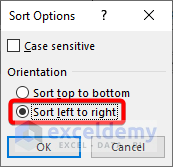
Choose Sort left to right from the Sort Options window that opens.
Click OK.

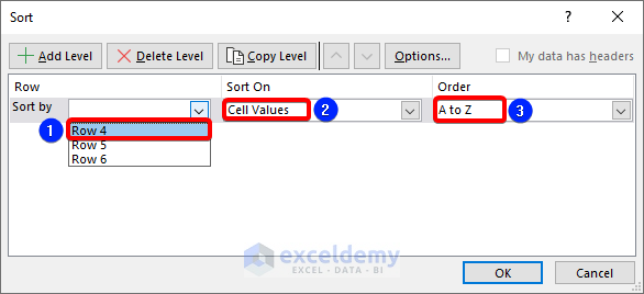
Click on the Sort by arrow and select Row 4 from the options.
Set Sort On to Cell Vales and Order to A to Z.

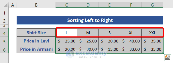
Row 4 is sorted in ascending alphabetical order from left to right, along with the rest of the dataset.

Method 3. Multi-Level Sorting in Excel

To sort multiple columns of a large database under specific conditions, we can use the Advanced Sorting option. We’ll use our main sample dataset for this method.

Steps:

Go to the Data tab and click Sort.
From the menu that appears, set Sort by to Region.
Set Order to A to Z.

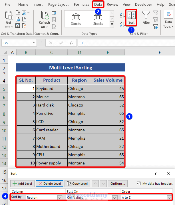
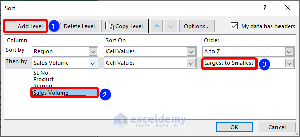
Now click the Add Level button and another option Then by appears.
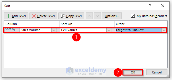
Select the Sales Volume option.
Select the Largest to Smallest option for Order.

Click OK.

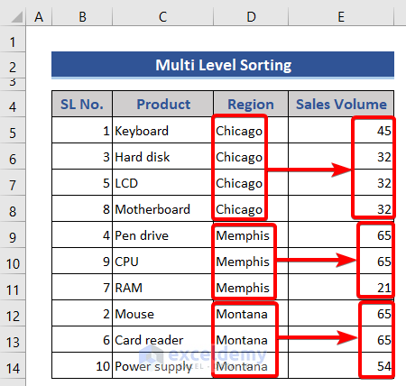
Our dataset is sorted first alphabetically by Region, and then in each Region by Sales Volume.

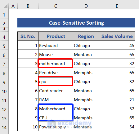
Method 4 – Case Sensitive Sorting

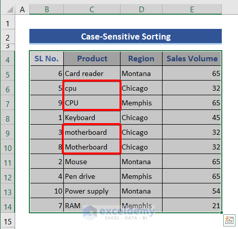
The Product column contains instances of the same product name but in different cases. Let’s sort them out.

Steps:

Select the whole dataset.
Go to the Data tab and click Sort.
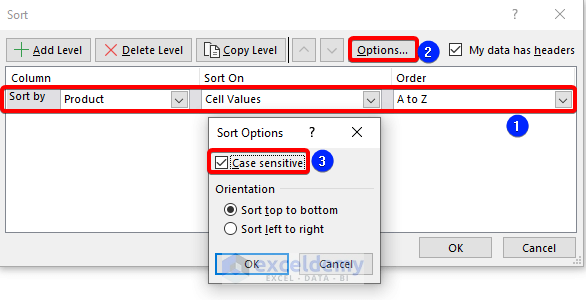
Select Product for Sort by, Cell Values for Sort On, and A to Z for Order.
Click on the Options button.
Check the Case sensitive box.
Click OK, then OK again.

The result of the Case Sensitive sorting is as follows:

Method 5 – Sorting by Cell Color and Font Color

Suppose our data contains cells with different fill colors. Let’s sort this data based on cell color or font color.

Steps:

Select the dataset and go to Data >> Sort.
Customize the Sort as follows: Sort by >> Region, Sort On >> Cell Color, Order >> Select any of the fill colors that appear in our data
Click OK.

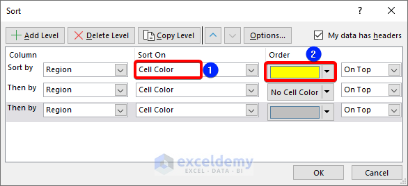
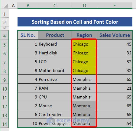
We added three levels to represent the three fill colors in our dataset.

Column D is now sorted by fill color, along with the rest of the dataset.

Method 6 – Advanced Sorting using Conditional Formatting

We can use Conditional Formatting to perform an advanced sort operation.

Steps:

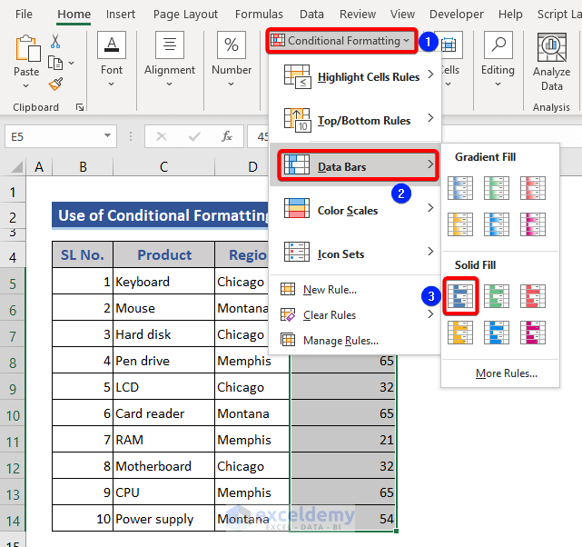
Select Column E.
From the Home tab, select Conditional Formatting >> Data Bars.
Choose a color from the Solid Fill section.

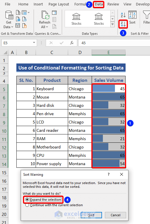
Bars are added to the data.

Go to Data >> Sort Largest to Smallest.
Choose Expand the selection from the Sort Warning window that opens.
Click on Sort.

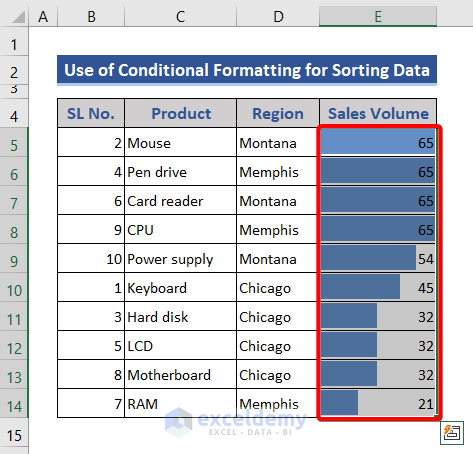
Our dataset is sorted by Sales Volume in descending order based on Color Formatting.

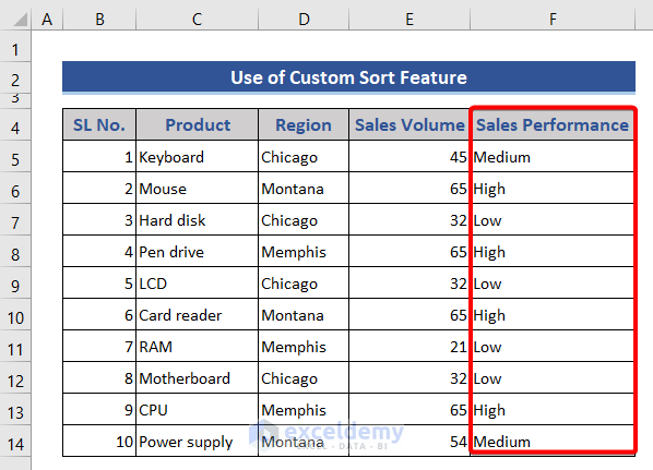
Example 7 – Sorting Based on a Custom List

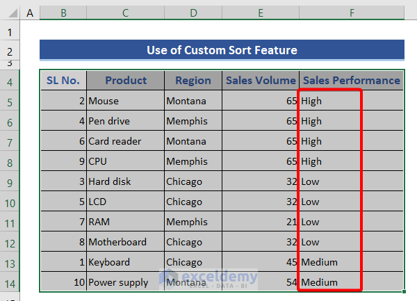
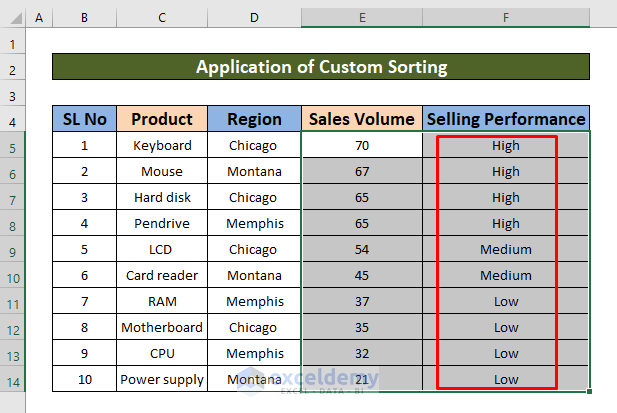
Suppose we give our products a Sales Performance value based on Sales Volume. Sales Volumes less than 40 are marked with Low performance; Sales Volumes greater than 40 but less than 60 are marked with Medium performance; and Sales Volumes greater than 60 are marked with High performance. Let’s sort by these values.

Steps:

Select the dataset.
From the Home tab, choose the Sort & Filter >> Custom Sort option.

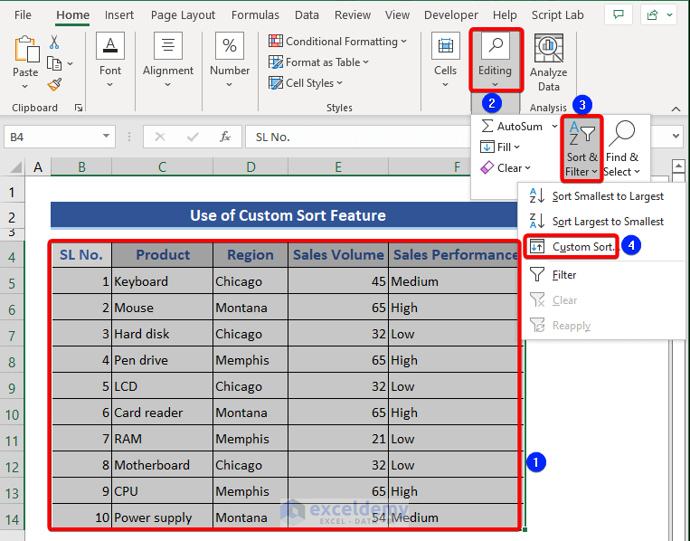
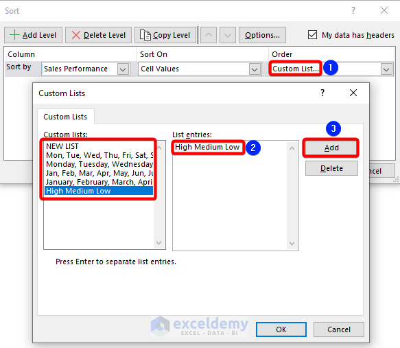
For Order, select Custom List.
In the Custom Lists box that opens, under Custom lists, select High Medium Low.
Under List entries, select High Medium Low.
Click Add.
Click on OK.

The dataset is sorted by the Sales performance column.

Method 8 – Using the SORT Function to Sort

The SORT Function is used to sort ranges or arrays. Let’s apply it to sort the data of Column E by Column F.

Enter the following formula in cell F5 to sort the whole column:

=SORT(E5:E14)

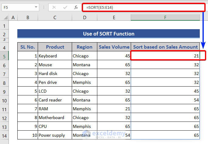
Our data sorted in ascending order.

Method 9 – Using the SORTBY Function for Advanced Sorting

The SORTBY function sorts a range or array based on the values in a corresponding range or array without changing the main data. Another benefit of this function is that it will sort data in ascending or descending order based on one of the ranges of the total sorting range. Let’s apply it.

Steps:

Consider the following the dataset:

The dataset is divided into two parts. the first before sorting, and the second after.

Enter the following formula in cell F6:

=SORTBY(B6:D15,D6:D15,-1)

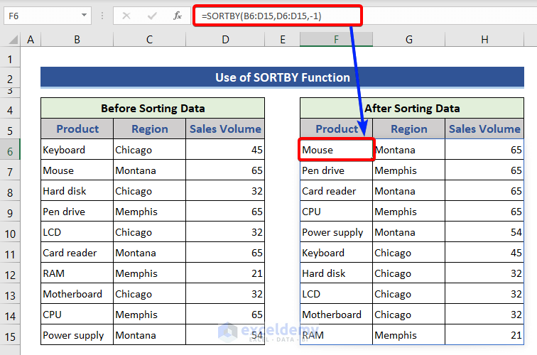
Our data is sorted by the Sales Volume column in descending order.

Download Practice Workbook

Advanced Sorting.xlsx

<< Go Back to Sort in Excel | Learn Excel

Get FREE Advanced Excel Exercises with Solutions!

2 Comments

Jack Jan 15, 2022 at 9:29 PM

In the last example, the table is supposed to be sorted by Selling performance (column E) using a custom order list. However, the result is not in the correct order. The column should be in the order: High Medium Low. Instead, it’s in standard alphabetical order.
Md. Abdur Rahim Rasel Aug 30, 2022 at 10:51 AM

Hello JACK,
You can easily do that using the Custom Sort command. Let’s follow the instructions below:
Let’s Sales volumes less than 40 are marked with low performance. Sales volumes greater than 40 but less than 60 are marked with medium performance. Sales volumes greater than 60 are marked with high performance.
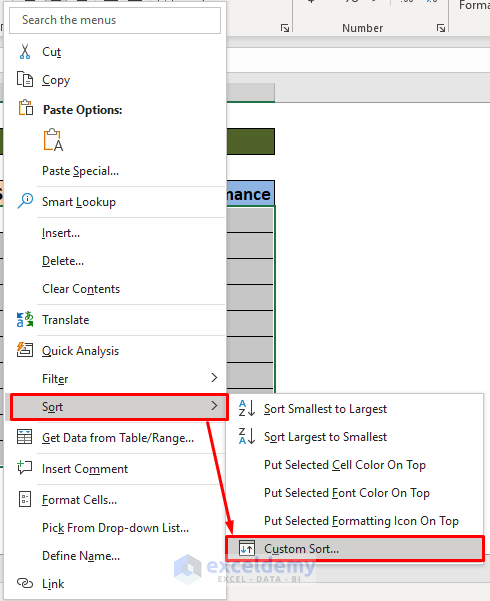
First of all, select cells range E5 to F14, and press right-click. As a result, a window pops up. From that window select Custom Sort under the Sort option.

After that, do like the below screenshot.

Finally, you will get your desired output.

Please download the below Excel file for your practice.
https://www.exceldemy.com/wp-content/uploads/2022/08/Advanced-Sorting-Options.xlsx
Thank you for your comment.
Regards
Md. Abdur Rahim Rasel(Exceldemy Team)