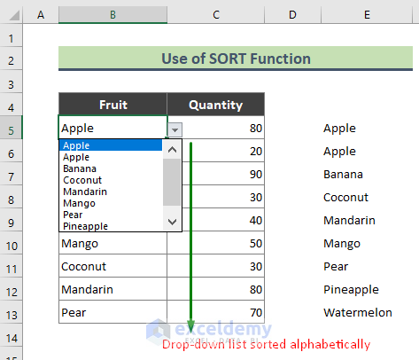
Method 1 – Applying the SORT Function to Arrange and Create a Drop-Down List
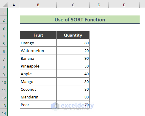
The sample dataset (B4:C13) contains fruit names in random order.
Steps:
- Enter this formula E5 and Press Enter.
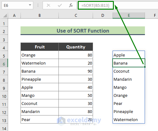
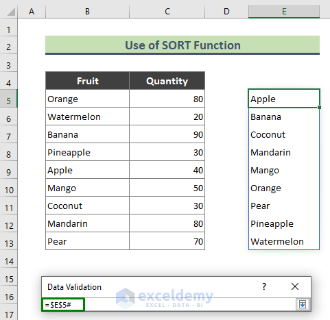
=SORT(B5:B13)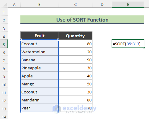
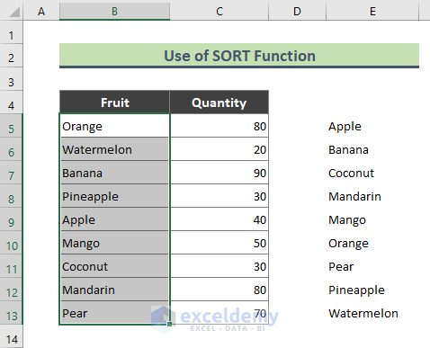
- The formula will sort data in ascending alphabetical order.
Creating a Drop-Down List:
Steps:
- Select any of the cells or the whole data range where you want to create the drop-down list.
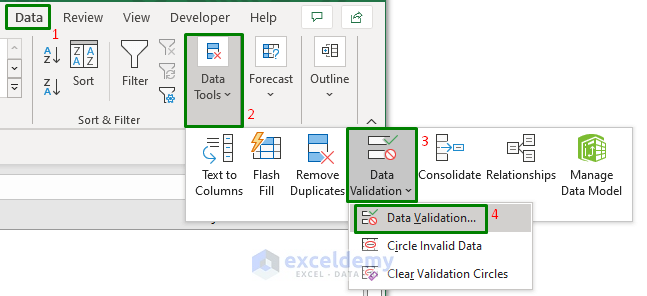
- On the Excel Ribbon, go to Data > Data Tools group > Data Validation > Data Validation
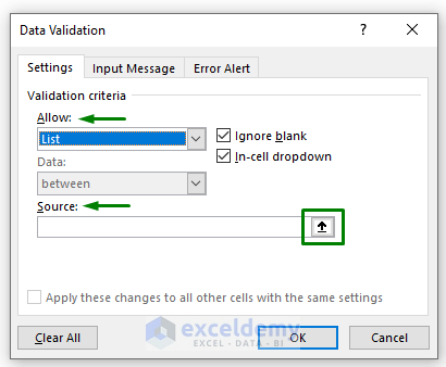
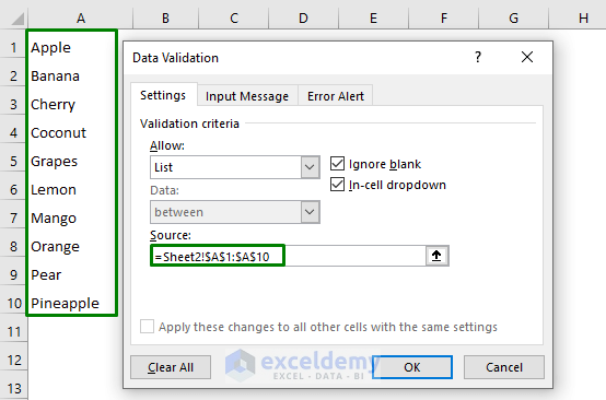
- In the Data Validation dialog box, choose List from the field: Allow. Source will be displayed. Click the upper arrow in the Source field to select the source data.
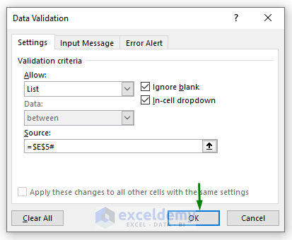
- Insert the source data and press Enter. ‘#’ was used at the end of the source data to include the whole array of the sorted data in the drop-down list.
- Click OK.
The drop-down list is created.
Read More: How to Sort and Filter Data in Excel
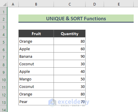
Method 2 – Combining the SORT & UNIQUE Functions to Sort a Drop-Down List
The dataset below contains Orange, Coconut, and Apple multiple times.
Steps:
- Enter the following formula in E5.
=UNIQUE(SORT(B5:B13))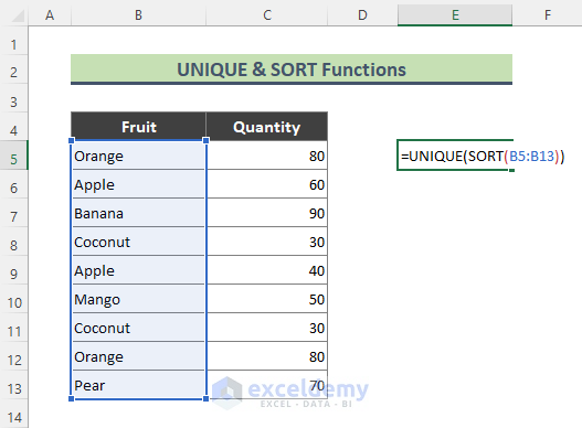
The array will contain unique fruit names.
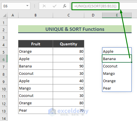
- Use the Data Validation option, to create the drop-down list.
Read More: How to Perform Random Sort in Excel
Method 3 – Using the OFFSET and COUNTA Functions with the Define Name Option to Organize the Drop-Down List
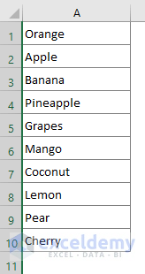
This is the sample dataset.
Steps:
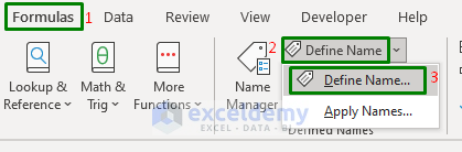
- Go to Formulas > Define Name > Define Name.
- The New Name dialog box will open. In Name enter Fruit.
- In Refers to, enter the formula below.
- Press OK.
=OFFSET(Sheet1!$A$1, 0, 0, COUNTA(Sheet1!$A$1:$A$1001))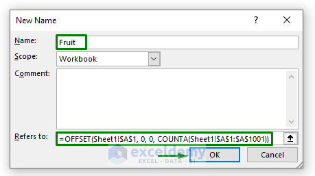
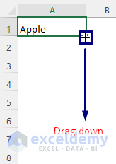
- Go to another sheet (Sheet2). Enter this formula in A1 and press Enter.
=IF(COUNTA(Fruit)>=ROWS($A$1:A1), INDEX(Fruit, MATCH(SMALL(COUNTIF(Fruit, "<"&Fruit), ROW(A1)),COUNTIF(Fruit, "<"&Fruit), 0)), "")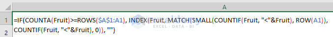
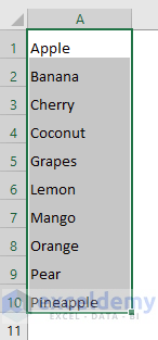
The formula will return a fruit name in alphabetical order. Drag down the ‘+’ sign to see the other fruit names.
The list is in alphabetical order.
- Create a drop-down list using the Data Validation option. Select the above list as source data.
Read More: How to Do Advanced Sorting in Excel
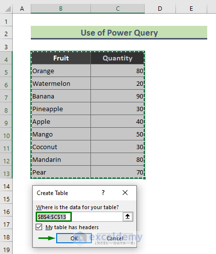
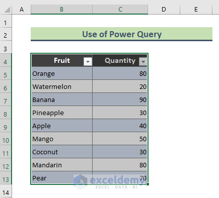
Method 4 – Applying the Excel Power Query to Sort Drop-down Data
The dataset was converted to a table by pressing Ctrl + T.
Steps:
- Select the table (B4:C13).
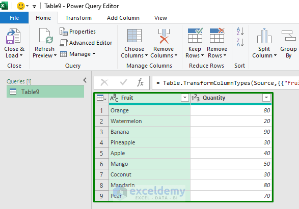
- Go to Data > From Table/Range.

- The Power Query Editor window will open.
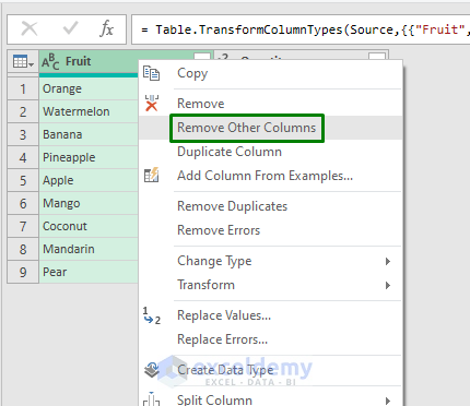
- Right-click the table and click Remove Other Columns.
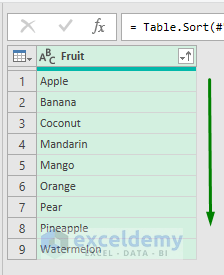
- Click the drop-down icon in the fruit column and click Sort Ascending.
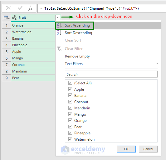
The fruit list will be sorted in alphabetical order.
- Select Close & Load > Close & Load in the Power Query Editor.
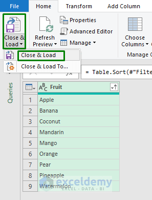
The table containing sorted fruit names is displayed.
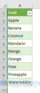
- Create the drop-down list.
Read More: How to Perform Custom Sort in Excel
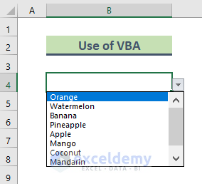
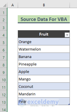
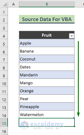
Method 5 – Ordering a Drop Down List Using VBA in Excel
This is the sample dataset.
Steps:
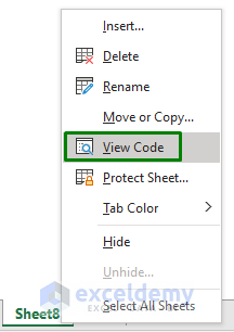
- Go to the sheet that contains the source data of the drop-down list. Here, Sheet8.
- Right-click the sheet name and select View Code.
- The Microsoft Visual Basic for Applications window will open. Enter the code below in the Module.
Option Explicit
Private Sub Worksheet_Change(ByVal Target As Range)
Dim rngSort As Range
'Set reference to the Table and column to be sorted
Set rngSort = ThisWorkbook.Worksheets("Sheet8").Range("FruitName[Fruit]")
'Use Range.Sort method to apply sort
rngSort.Sort _
Key1:=rngSort, _
Order1:=xlAscending, _
Header:=xlYes
End Sub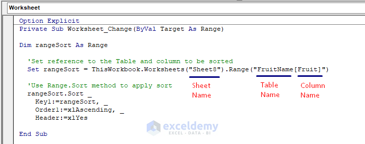
- Go to the source data table and enter any fruit name, like ‘Dates’, in B14.
- Press Enter.
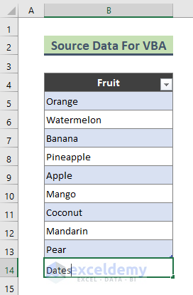
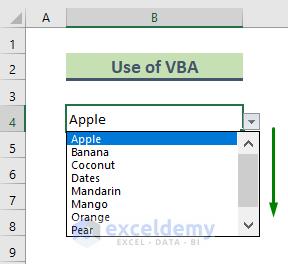
- Data is sorted alphabetically.
The drop-down list is also sorted in alphabetical order.
Read More: Advantages of Sorting Data in Excel
Download Practice Workbook
Download the practice workbook.
Related Articles
<< Go Back to Sort in Excel | Learn Excel
Get FREE Advanced Excel Exercises with Solutions!
