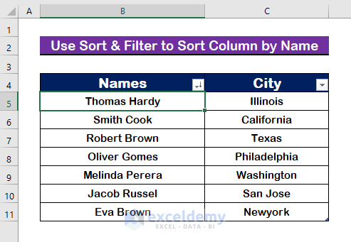
Example 1 – Use Sort & Filter Group to Sort Columns by Name
To sort names alphabetically.
1.1 Sort a Column by Name
Step 1:
- Select the first cell which contains a person’s name.
Step 2:
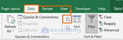
- From the Ribbon, choose the Data tab.
- Click on the A → Z icon from the Sort & Filter group.
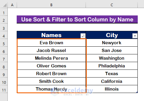
You will get the column with a sorted value as shown in the image.
1.2 Sort Multiple Columns by Name
Step 1:
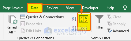
- Click on the Data tab from the Ribbon.
- From the Sort & Filter group, select Sort.
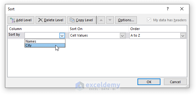
Step 2:
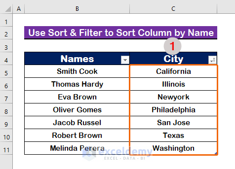
- From the table, choose any of your preferred columns to sort by. We have chosen City to sort it.
- You will get the sorted value according to the second column.
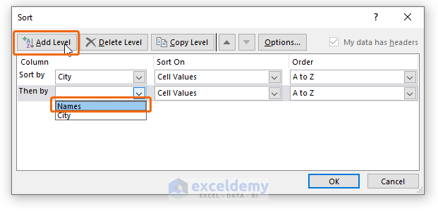
Step 3:
- To sort by another column, click on the Add Level.
- From the They by list, choose the column listed as Names.
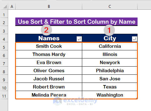
Step 4:
- Press OK.
Read More: How to Sort by Last Name in Excel
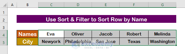
Example 2 – Use Sort & Filter Group to Sort Rows by Name
You may sort a row by names in addition to sorting by columns. We have reorganized the Names and City values in a row.
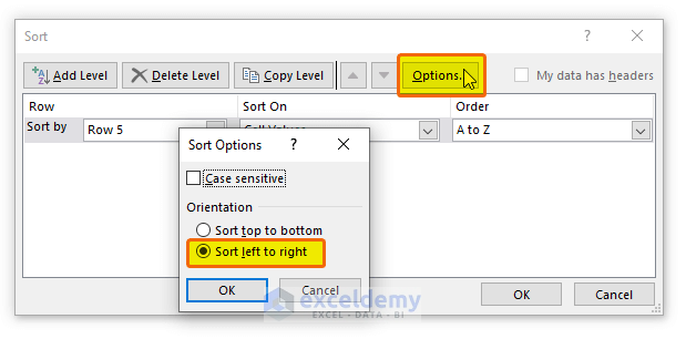
Step 1:
- After opening the Sort option from the Sort & Filter group, click on the Options tab.
- Select Sort left to right.
- Press OK.
Step 2:
- From the Sort by menu, choose Row 4.
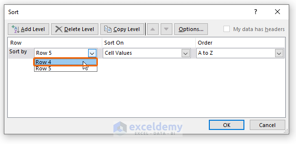
Step 3:
- Press Enter to see the results.
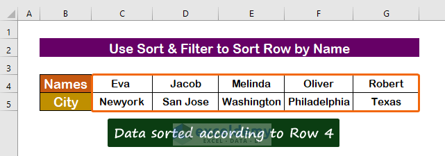
Notes. You can sort the data according to any of your existing rows.
Read More: How to Sort Numbers in Excel
Example 3 – Apply Formula to Sort by Name
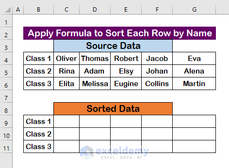
3.1 Apply Formula to Sort Each Row by Name
Steps:
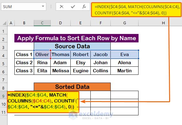
- In the desired cell, enter the following formula for the first row in range C4:G4.
=INDEX($C4:$G4, MATCH(COLUMNS($C4:C4), COUNTIF($C4:$G4, “<=”&$C4:$G4), 0))
- The COUNTIF function will return by counting serially the match between C4:G4.
- The MATCH function provides the match between columns.
- The INDEX function will give us the matched result serially.
- To make it work as an array, press Ctrl + Shift + Enter
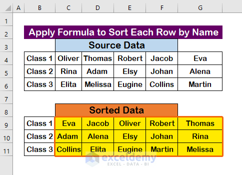
- Use the AutoFill tool to fill up the required cells.
- The rows will be sorted individually as shown in the image below.
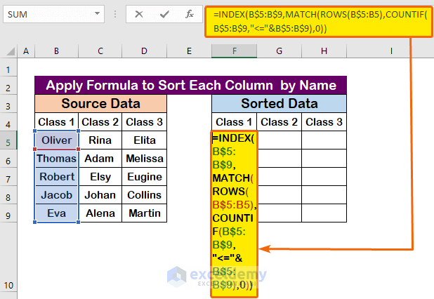
3.2 Apply Formula to Sort Each Column by Name
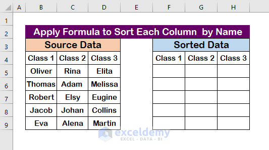
Steps:
- In F5, enter the following formula for the range B5:B9.
=INDEX($C4:$G4, MATCH(COLUMNS($C4:C4), COUNTIF($C4:$G4, “<=”&$C4:$G4), 0))
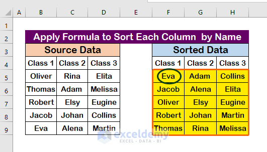
- To make it work as an array, press Ctrl + Shift + Enter
- Use AutoFill for the remaining cells.
- The data in each column will be sorted alphabetically by names.
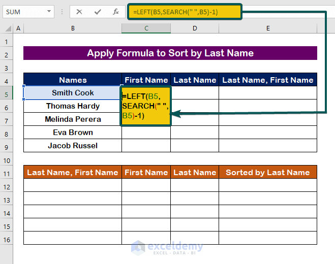
3.3 Apply Formula to Sort by Last Name
Step 1:
- To separate the First Names from the Names, enter the following formula.
=LEFT(B5,SEARCH(” “,B5)-1)
- The SEARCH function finds the space in B5.
- The LEFT function returns the remaining value after space found from the SEARCH.
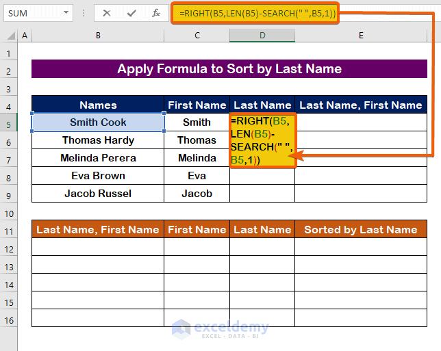
Step 2:
- To separate the Last Name, enter the following formula.
=RIGHT(B5,LEN(B5)-SEARCH(” “,B5,1))
Step 3:
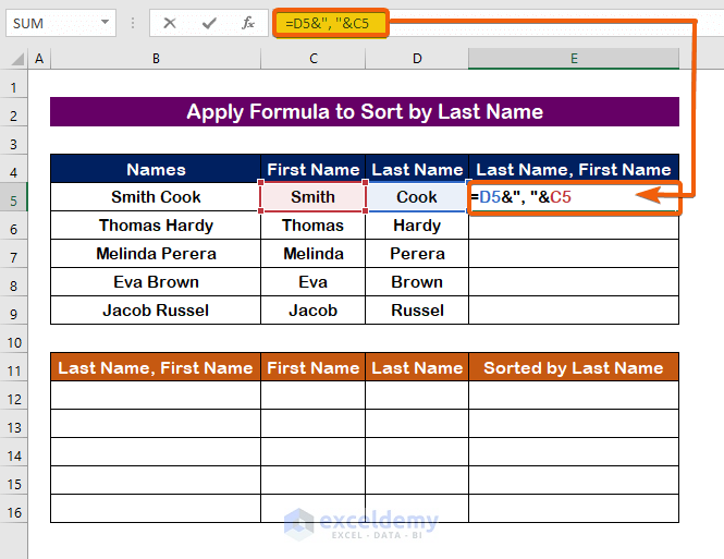
- To add the Last Name first and the First Name last, enter the following formula.
=D5&”, “&C5
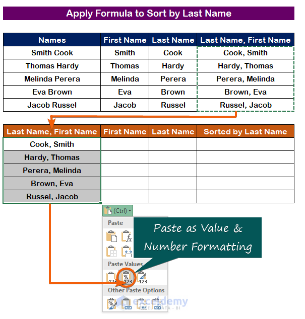
Step 4:
- In the desired cell, copy the cells and paste them as Value & Number Formatting.
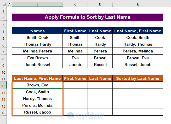
Step 5:
- From the Data tab, click on the icon shown in the image below.

- The data will be sorted by their last names.
Step 6:
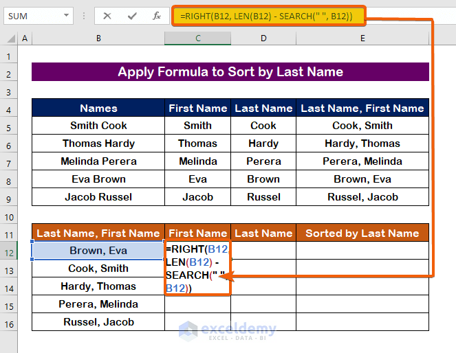
- Enter the following formula to keep only the First Name.
=RIGHT(B12, LEN(B12) – SEARCH(” “, B12))
- In cell C12, the RIGHT function provides the value from the B12 cell with the number of characters left from applying the SEARCH function after space.
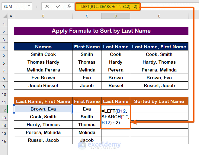
Step 7:
- Enter the following formula to keep the Last Name.
=LEFT(B12, SEARCH(” “, B12) – 2)
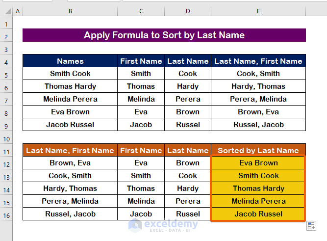
Step 8:
- Combine both cells with the following formula.
=C12&” “&D12
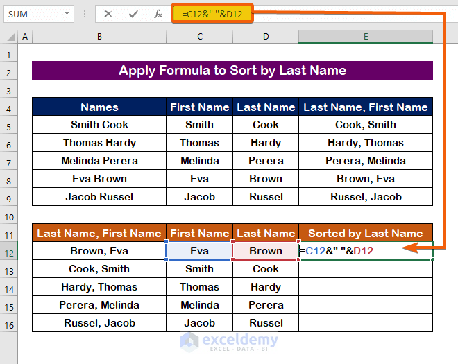
- The data will be sorted by their last names.
Read More: How to Sort in Excel by Number of Characters
Download Practice Workbook
Related Articles
- How to Sort Duplicates in Excel
- How to Sort Unique List in Excel
- How to Sort Merged Cells in Excel
- How to Sort Merged Cells of Different Sizes in Excel
- How to Put Numbers in Numerical Order in Excel
- How to Arrange Numbers in Ascending Order in Excel Using Formula
<< Go Back to Sort in Excel | Learn Excel
Get FREE Advanced Excel Exercises with Solutions!
