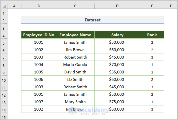
The sample dataset showcases Employee Name, ID No., Salary & Rank.
Method 1 – Getting a Sorted Unique List
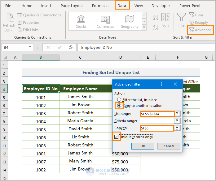
1.1. Using the Advanced Filter
- Select the whole dataset.
- Go to Data tab > Choose Advanced in Sort & Filter.
- Set the List range as $C$5:$C$14.
- Keep the Criteria range blank.
- Check Copy to another location.
- Check Unique records only.
- Click OK.
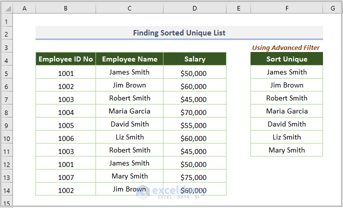
This is the output.
1.2. Combination of the SORT & UNIQUE Functions
- Use the following formula:
=SORT(UNIQUE(C5:C14))
C5:C14 is the cell range for the name of the employee.
The UNIQUE(C5:C14) syntax returns unique values and the SORT function sorts the found unique values in ascending order.
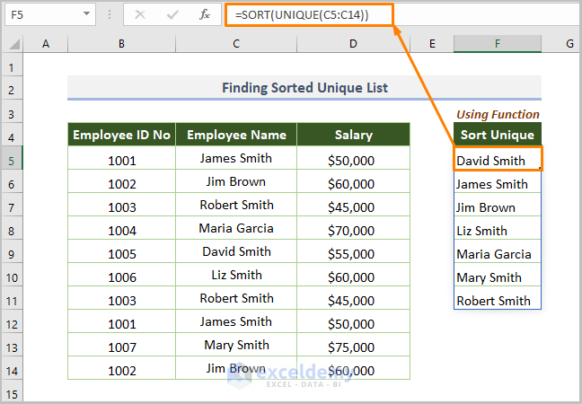
The above picture is the output.
Read More: How to Sort by Last Name in Excel
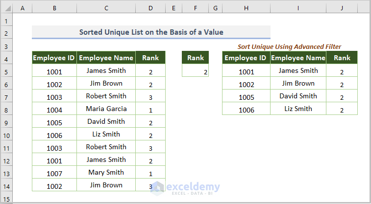
Method 2 – Sorting a Unique List Based on a Value
2.1. Using the Advanced Filter
- In the Advanced Filter dialog box, set the List range as $B4:$D14 and the Criteria range as $F4:$F5.
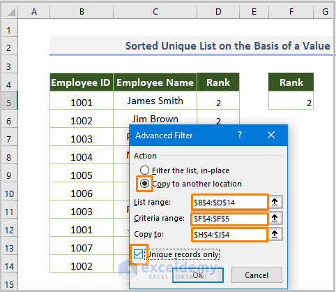
- Click OK to see the output.
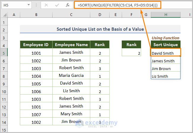
2.2. Using Function
- Use the following formula:
=SORT(UNIQUE(FILTER(C5:C14, F5=D5:D14)))
C5:C14 is the cell range for the name of the employee, F5 is the given value, and D5:D14 is the cell range for the Rank field.
In the FILTER function, C5:C14 is set as an array. F5=D5:D14 includes the specific value.
The UNIQUE function returns the unique value of the filtered data.
The SORT function sorts the found unique values in ascending order.
- Press Enter to see the output.
Read More: How to Sort Duplicates in Excel
Method 3 – Sorting a Unique List Based on a Cell Range
3.1. Using Advanced Filter
- In the Advanced Filter dialog box, set the List range as $B$4:$D$14 and the Criteria range as $F$4:$G$5.
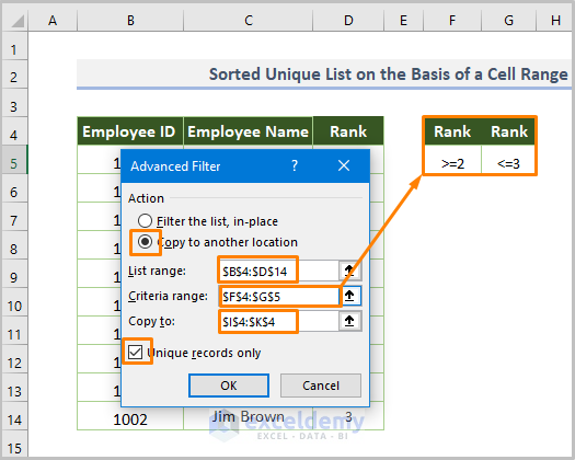
This is the output.
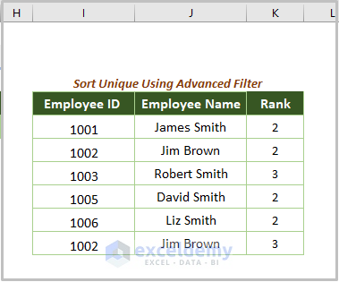
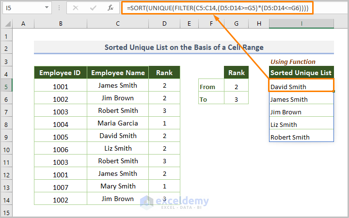
3.2. Using a Function
- Enter the following formula.
=SORT(UNIQUE(FILTER(C5:C14,(D5:D14>=G5)*(D5:D14<=G6))))
C5:C14 is the cell range for the name of the employee, G5 is the given first value, G6 is the second value, and D5:D14 is the cell range for Rank field.
Read More: How to Sort by Name in Excel
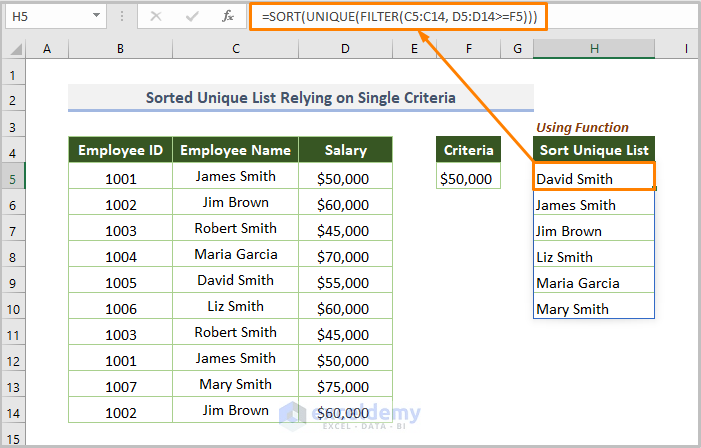
Method 4 – Sorting a Unique List Based on a Single Criterion
To sort unique values if the salary is greater than or equal to $50000.
4.1. Using the Advanced Filter
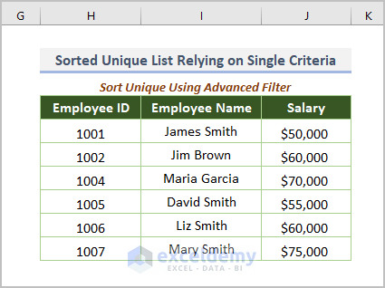
- In the dialog box, specify the List range as $B$4:$D$14 and the Criteria range as $F$4:$F$5.
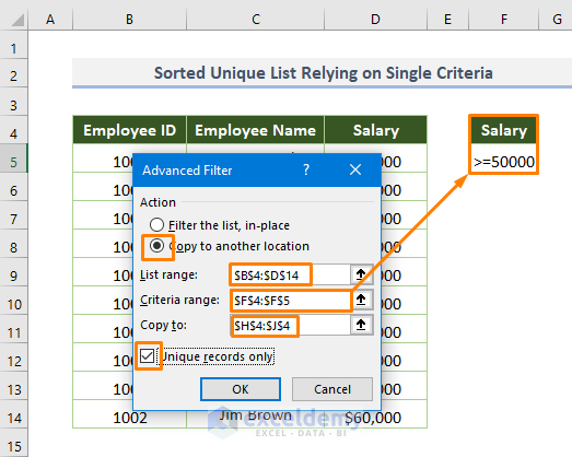
This is the output.
4.2. Using a Function
- Enter the formula below.
=SORT(UNIQUE(FILTER(C5:C14, D5:D14>=F5)))
C5:C14 is the cell range for the name of the employee, F5 is the given value, and D5:D14 is the cell range for the Rank field.
Method 5 – Sorting a Unique List Based on Multiple Criteria
To sort the dataset for a salary greater than or equal to $50000 and for a rank equal to 2:
5.1. Using the Advanced Filter
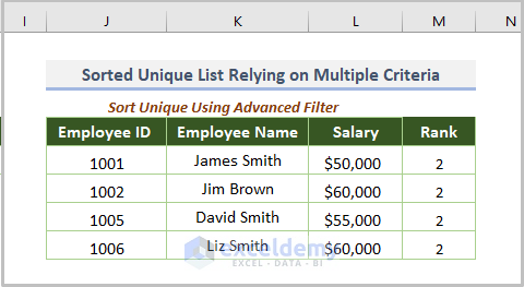
- In the dialog box, set the List range as $B$4:$E$14 and the Criteria range as $G$4:$H$5.
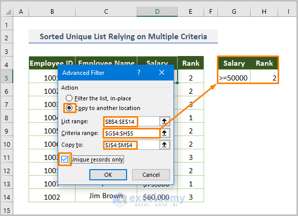
This is the output.
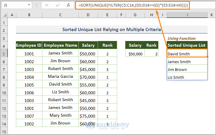
5.2. Using a Function
- Enter the following formula.
=SORT(UNIQUE(FILTER(C5:C14,(D5:D14>=G5)*(E5:E14=H5))))
C5:C14 is the cell range for the name of the employee, G5 is the required salary, H5 is the second value, D5:D14 is the cell range for the Salary field, and E5:E14 is the cell range for the Rank field.
Read More: How to Arrange Numbers in Ascending Order with Excel Formula
Method 6 – Creating a Dynamic Sorted Unique List
- Select the entire dataset.
- Go to the Insert tab > click Table.
- Check My table has headers.
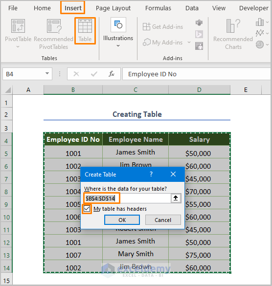
- The created table (Table1) with the source data is stored in Excel.
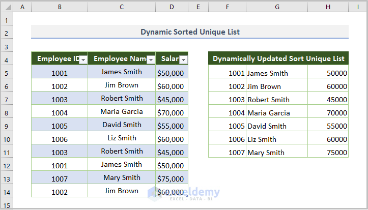
- Enter the following formula.
=SORT(UNIQUE(Table1))
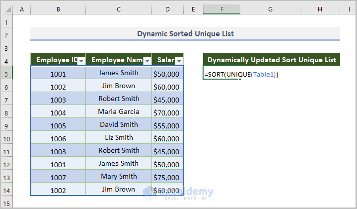
- Press Enter to see the dynamic list of the sorted unique data.
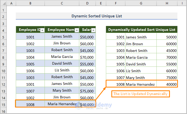
- Enter new data (ID: 1008) and the list is automatically updated.
Read More: How to Sort Merged Cells in Excel
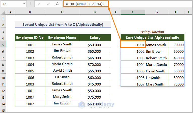
Method 7 – Sorting a Unique List from A to Z (Alphabetically)
- Enter the formula:
=SORT(UNIQUE(B5:D14))
B5:D14 is the dataset.
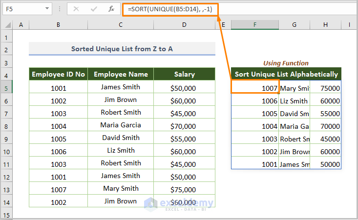
Method 8 – Sorting a Unique List from Z to A
- Enter this formula:
=SORT(UNIQUE(B5:D14), ,-1)
B5:D14 is the dataset, and -1 is the descending order.
Read More: How to Sort in Excel by Number of Characters
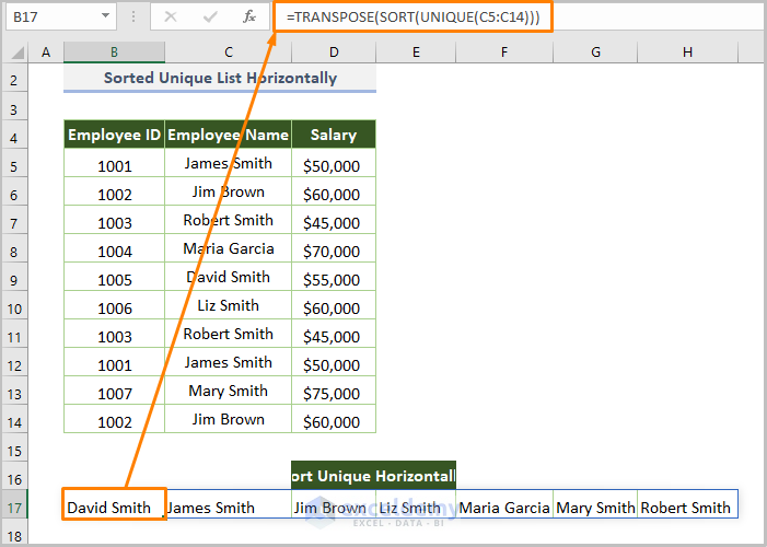
Method 9 – Sort the Unique List Horizontally
- Use this formula.
=TRANSPOSE(SORT(UNIQUE(C5:C14)))
C5:C14 is the name of the employee.
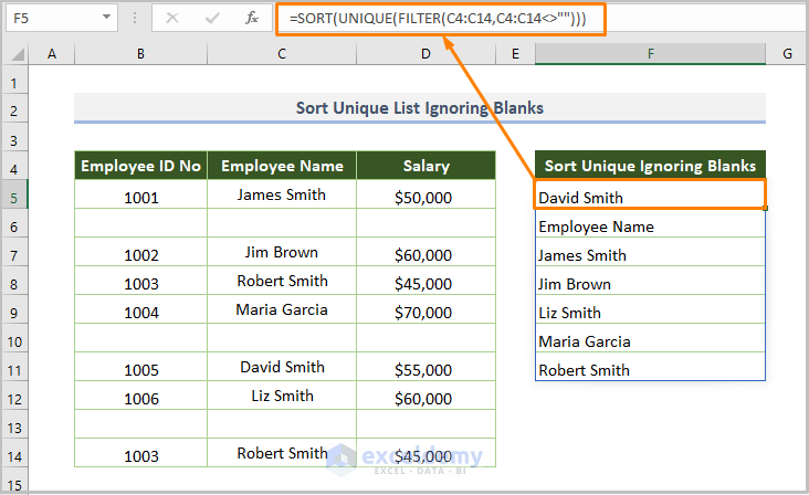
Method 10 – When Some Cells are Blank
To ignore blank cells and sort the unique list in Excel:
- Enter the formula.
=SORT(UNIQUE(FILTER(C4:C14,C4:C14<>"")))
C4:C14 is the name of the employee, ” ” ignores blank cells.
Things to Remember
| Name of Errors | When Occurs |
|---|---|
| #CALC! | If the UNIQUE function cannot extract the unique values. |
| #SPILL! | If there is any value in the spill range from which the UNIQUE function will return the list. |
| #VALUE! | If the output (sorted unique values) is not available in the given dataset. |
Download Practice Workbook
Related Articles
- How to Sort Numbers in Excel
- How to Put Numbers in Numerical Order in Excel
- How to Sort Merged Cells of Different Sizes in Excel
<< Go Back to Sort in Excel | Learn Excel
Get FREE Advanced Excel Exercises with Solutions!

Excellent Work – thank you.
Hello Mo Sheikh,
You are most welcome. Thanks for your feedback and appreciation. Keep learning Excel with ExcelDemy!
Regards
ExcelDemy