Method 1 – Arranging Numbers in Ascending Order in Excel Using SMALL with ROWS and COLUMNS Functions
1.1 Sorting by Rows
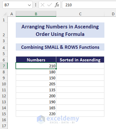
Combine SMALL with the ROWS function to sort numbers by rows and arrange them in ascending order.
In the following dataset, you have some random numbers. Arrange these numbers in ascending order using a formula.
Follow the steps below to perform the task.
Steps:
- Select cell C7 => Insert the formula:
=SMALL($B$7:$B$15,ROWS($B$7:B7))- Press Enter.
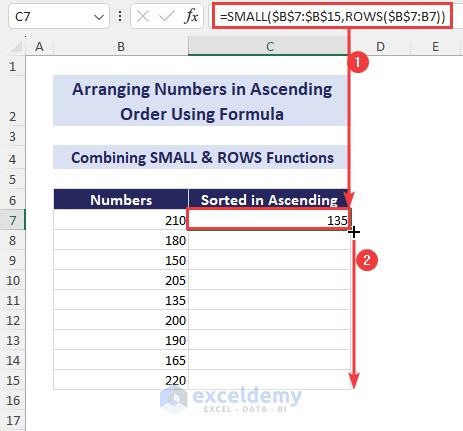
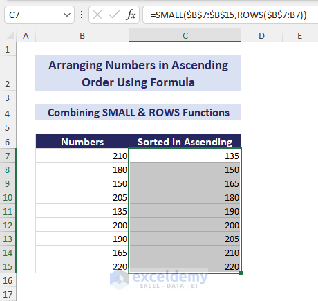
- Use the Fill Handle to copy the formula in the other cells below. It will return the numbers in ascending order.
Combine the AGGREGATE & ROWS functions, arranging numbers in ascending order. We’ll get the same output as shown above. The formula will be:
=AGGREGATE(15,0,$B$7:$B$15,ROWS($B$7:B7))1.2 Sorting by Columns
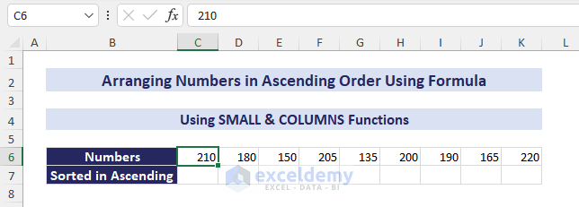
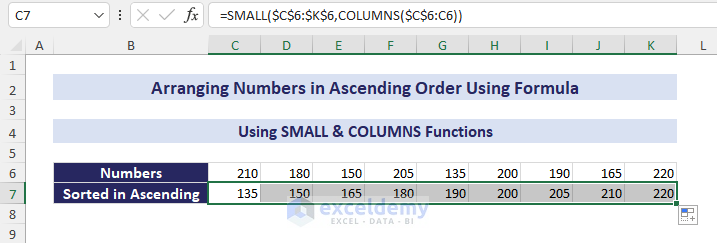
Combine SMALL with the COLUMNS function to sort numbers by columns and arrange them in ascending order.
In the following dataset, we have some random numbers in row 6. Arrange these numbers in ascending order in row 7.
Follow the steps below.
Steps:
- Select cell C7 => Write the formula:
=SMALL($C$6:$K$6,COLUMNS($C$6:C6))- Press Enter.
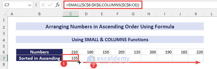
- Use the Fill Handle to copy the formula into other cells on the right side. It will return the numbers in ascending order.
Method 2 – Using SORT Function to Arrange Numbers in Ascending Order Along with Dataset
2.1 Sorting by Rows
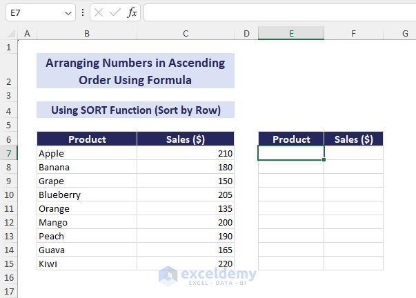
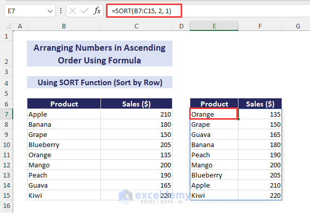
Use the Excel SORT function to sort by rows and arrange numbers in ascending order along with the dataset.
You have some products and sales in dollars. Arrange the products based on the ascending order of sales.
Learn the following steps.
Steps:
- Select cell E7 => Type the formula:
=SORT(B7:C15, 2, 1)- Press Enter. It’ll spill the dataset in ascending order.
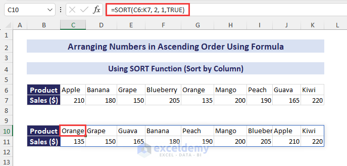
2.2 Sorting by Columns
Steps:
- Select cell C10 => Write the formula:
=SORT(C6:K7, 2, 1,TRUE)- Press Enter. It’ll spill the dataset in ascending order.
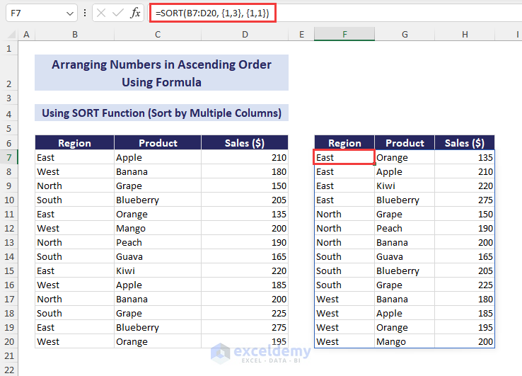
2.3 Sorting by Multiple Columns
Insert the SORT function to sort by multiple columns to arrange numbers in ascending order in Excel.
The following dataset includes some regions, products, and sales. Arrange the dataset in ascending order of regions and sales.
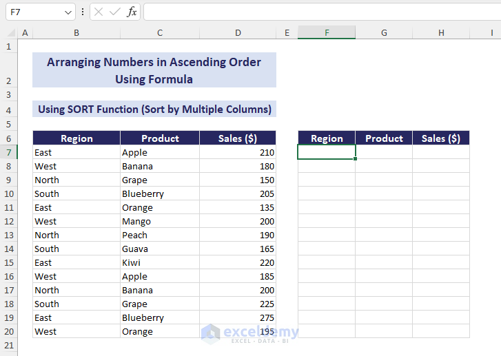
Follow the steps below to accomplish the task.
Steps:
- Select cell F7 => Type the formula:
=SORT(B7:D20, {1,3}, {1,1})- Press Enter to spill the output. See the regions in ascending order, and the sales are also in ascending order in each region.
2.4 Sorting N Smallest Values
Use the SORT function with the INDEX and SEQUENCE functions to arrange N smallest numbers in ascending order along with the dataset.
You have some products and sales in dollars. Input the desired number for N in F6, and later sort and extract data of the N smallest sales values in ascending order.
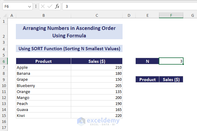
Learn the steps below.
Steps:
- Select cell E10 => Type the formula:
=INDEX(SORT(B7:C15, 2, 1 ), SEQUENCE(F6), {1,2})- Press Enter. It’ll spill the data of the N smallest sales in ascending order.
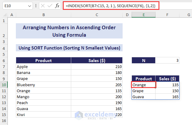
The following GIF shows the sorting of the data corresponding to the change in the value of N in F6.
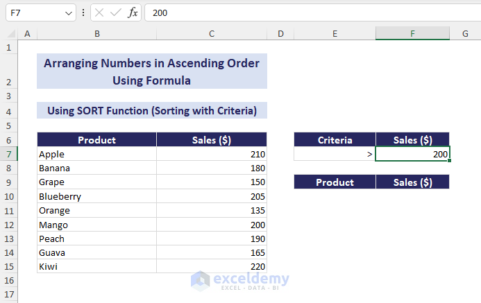
2.5 Sort and Filter (Sorting with Criteria)
Apply the SORT function with the IFERROR and FILTER functions to sort with criteria and arrange numbers in ascending order.
You have some products and sales. We’ll sort only the products that meet specified criteria. Arrange in ascending order only those products whose sales are greater than $200.
Follow the steps below to perform the task.
Steps:
- Select cell E10 => Type the formula:
=IFERROR(IF(E7=">=", SORT(FILTER(B7:C15, C7:C15>=F7), 2), IF(E7=">",SORT(FILTER(B7:C15, C7:C15>F7),2), IF(E7="=",SORT(FILTER(B7:C15, C7:C15=F7),2), IF(E7="<=",SORT(FILTER(B7:C15, C7:C15<=F7),2), SORT(FILTER(B7:C15, C7:C15<F7),2))))), "")- Press Enter to spill the output. See the desired products in ascending order.
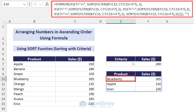
The following GIF shows the change in formula output whenever we change the criteria. It’ll arrange the numbers in ascending order accordingly.
2.6 Dynamic Sorting with Table
Use the SORT function along with the Table feature to sort dynamically, including any new entry, and arrange in ascending order accordingly.
The methods we have described can capture changes in the existing dataset. However, when you add new entries after the last row of the dataset, they are not included in the formula output. This method will use the Table feature to overcome that issue.
Follow the steps to accomplish the task.
Steps:
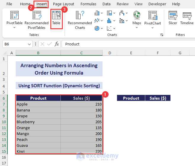
- Select the range B6:C15.
- Go to Insert => Click Table.
The Create Table dialog box pops out.
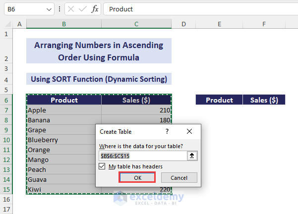
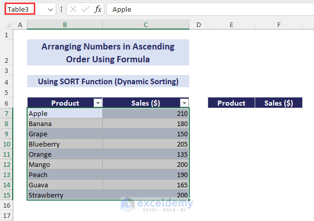
- Press OK in the dialog. The cell range will be converted into a table. Table 3 is the newly created table name.
- Select cell E7 => type the formula:
=SORT(Table3, 2, 1)- Press Enter. It’ll spill the formula output.

The following GIF shows the addition of a new product Kiwi to the main dataset. The formula output also gets updated accordingly and places the product in an accurate order.
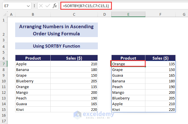
Method 3 – Applying SORTBY Function to Sort Numbers in Ascending Order in Excel
Arrange numbers in ascending order in Excel with the SORTBY function.
The SORTBY function is available only in Microsoft 365 and Excel 2021.
Steps:
- Select cell E7 => Insert the formula:
=SORTBY(B7:C15,C7:C15,1)- Press Enter. It’ll spill the outputs in ascending order.
Download Practice Workbook
<< Go Back to Sort Numbers | Sort in Excel | Learn Excel
Get FREE Advanced Excel Exercises with Solutions!
