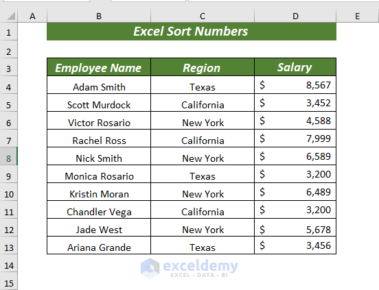
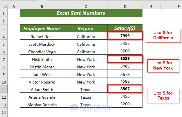
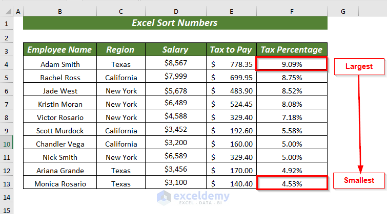
We’ll use a sample dataset that contains the salary information of a particular employee with the Employee Name, Region, and Salary columns.
How to Sort Numbers in Excel (8 Easy Ways)
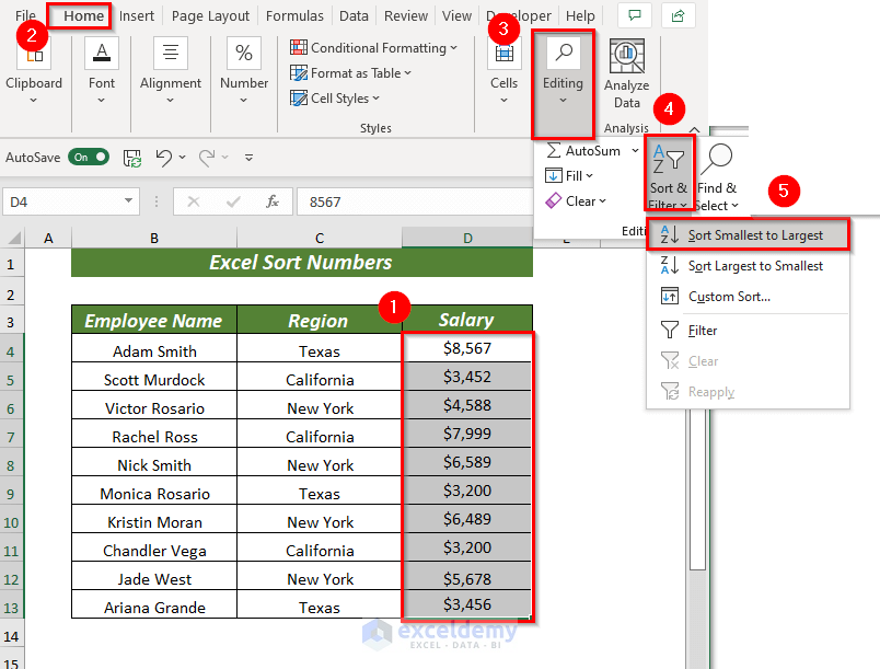
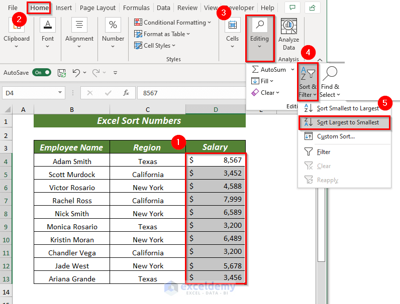
Method 1 – Sort Numbers from Smallest to Largest in Excel
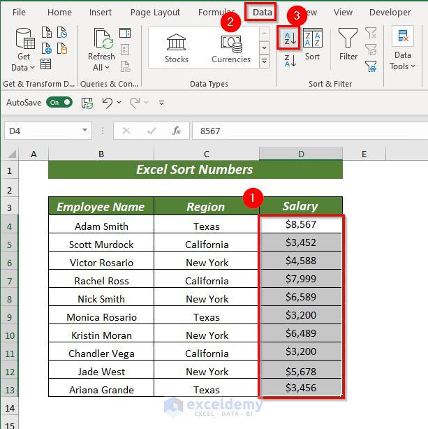
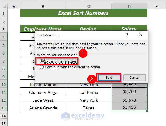
- Select the cell range that contains numbers. We selected the cell range D4:D13.
- Open the Home tab.
- Go to Editing.
- From Sort & Filter, select Sort Smallest to Largest.
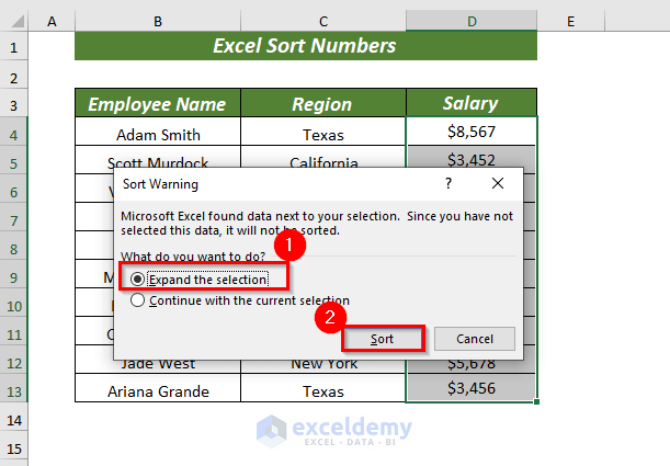
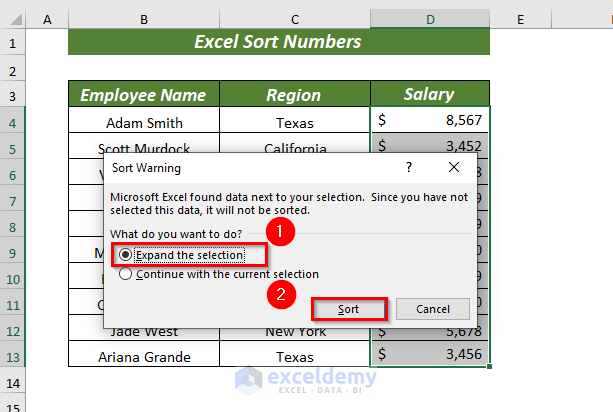
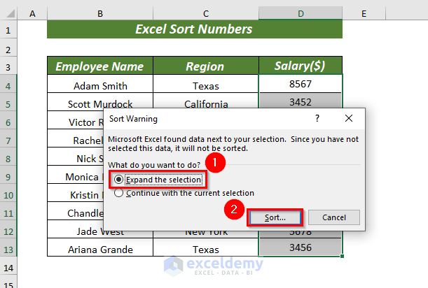
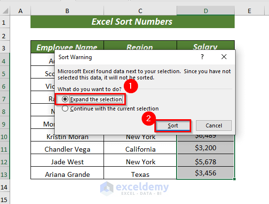
- A dialog box will pop up. Select Expand the selection.
- Click on Sort.
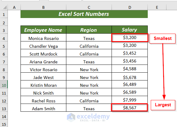
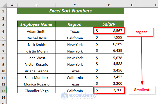
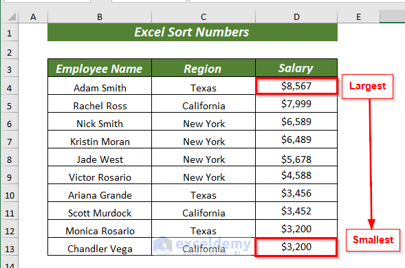
- This will Sort the numbers in the ascending order by moving entire rows around.
Read More: How to Arrange Numbers in Ascending Order with Excel Formula
Method 2 – Sort Numbers from Largest to Smallest in Excel
- Select the cell range that contains numbers. We selected the cell range D4:D13.
- Open the Home tab.
- Go to Editing.
- From Sort & Filter, select Sort Smallest to Largest.
- A dialog box will pop up. Select Expand the selection.
- Click on Sort.
- This will Sort the numbers in descending order along with the adjacent cell values.
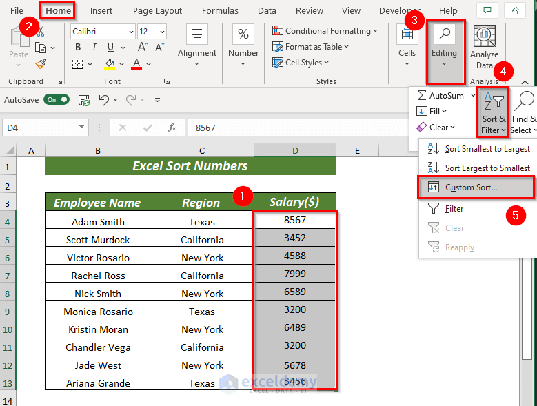
Method 3 – Sort Numbers Based on Criteria in Excel
- Select the cell range that contains numbers. We selected the cell range D4:D13.
- Open the Home tab.
- Go to Editing.
- From Sort & Filter, select Custom Sort.
- A dialog box will pop up. Select Expand the selection.
- Click on Sort.
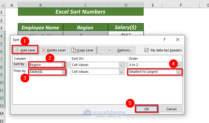
- Another dialog box will pop up. Click on Add Level
- In Sort by, select the Column name to sort first. We chose the Region column in Sort by selected A to Z.
- In Then by, select the Column which contains the numbers. We selected the Salary($) column in Then by and chose Smallest to Largest.
- Click on OK.
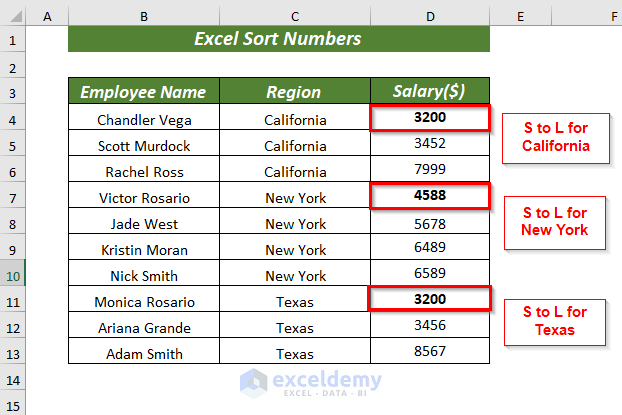
- This will Sort the values based on the Region column (alphabetically from A to Z), then in ascending order within each region.
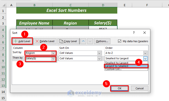
You can also Sort numbers by region and then in the descending order.
- Choose the Region column in Sort by and, in Order, select A to Z.
- Choose the Salary($) column in Then by and, in Order, select Largest to Smallest.
- Click on OK.
- Here are the results.
You can use the Sort command from the Data tab to use Custom Sort. Open the Data tab and select Sort.
Read More: How to Put Numbers in Numerical Order in Excel
Method 4 – Using Excel Formula to Sort Numbers in Ascending Order
- We named the range D4:D13 as data_1.
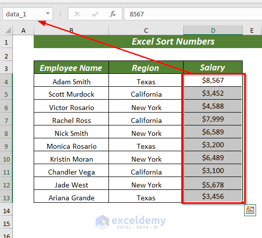
- Select any cell to place the resulting value. We selected cell F4.
- Insert the following formula.
=SMALL(data_1,ROWS($D$4:D4))
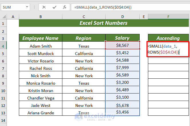
The SMALL function will extract the Smallest number from the given range of data.
- Press Enter.
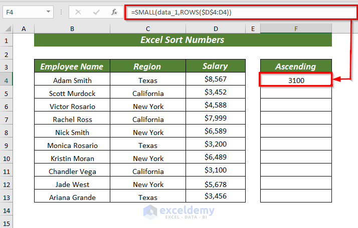
- Use the Fill Handle to autofill the formula for the rest of the cells.
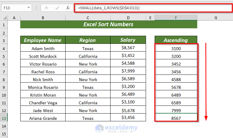
Here, all the numbers are sorted in ascending order.
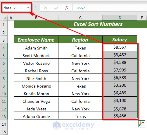
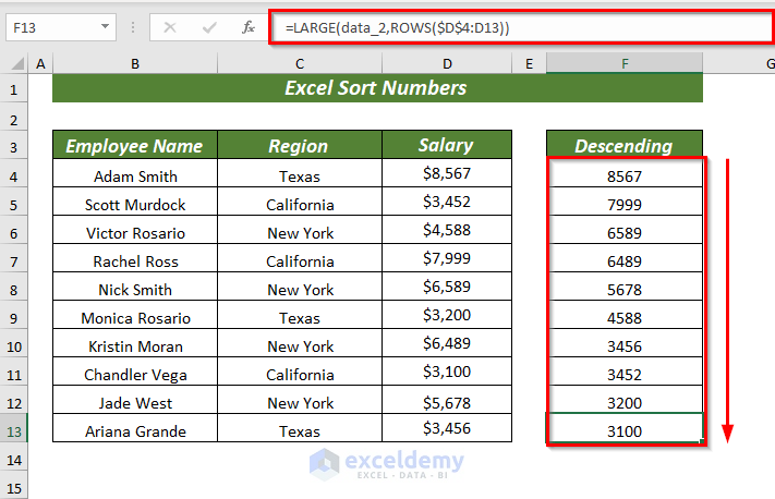
Method 5 – Using Excel Formula to Sort Numbers in Descending Order
- We named the range D4:D13 as data_2.
- Select any cell to place the results. We chose the cell F4.
- Insert the following formula.
=LARGE(data_2,ROWS($D$4:D4))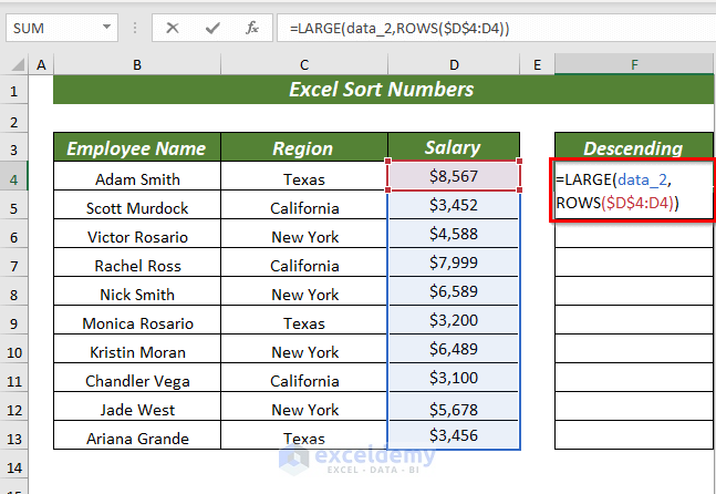
- Press Enter.
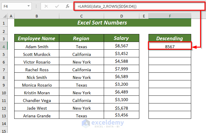
- Use the Fill Handle to AutoFill the formula for the rest of the cells.
Method 6 – Sort Numbers Using the Context Menu
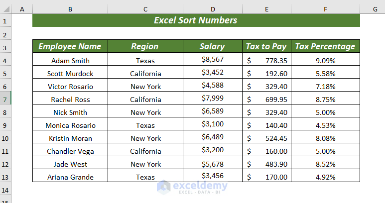
We added two columns, Tax to Pay and Tax Percentage, to show you how different Number Formats work while Sorting.
- Select the cell range from which you want to sort the numbers. We selected the cell range F4:F13.
- Right-click and choose Sort, then select Sort Largest to Smallest.
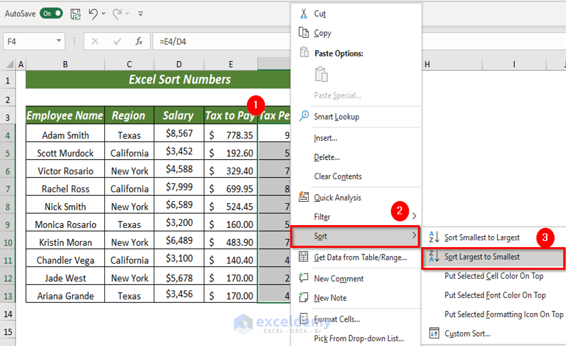
- A dialog box will pop up. Select Expand the selection.
- Click on Sort.
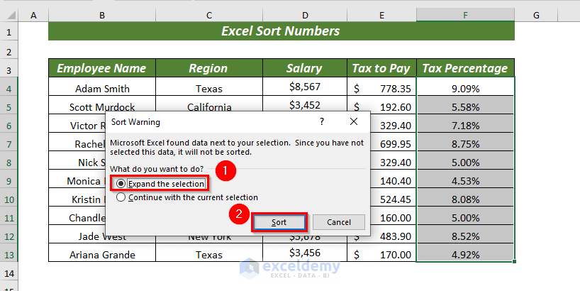
- This will Sort the numbers in descending order along with the adjacent cells’ values.
Read More: How to Sort Duplicates in Excel
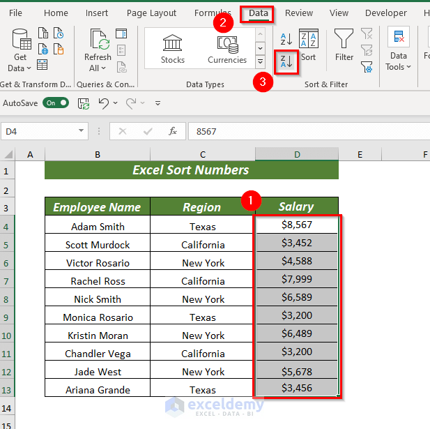
Method 7 – Using the A→Z Command to Sort Numbers from Smallest to Largest
- Select the cell range that contains numbers. We selected the cell range D4:D13.
- Open the Data tab and select A→Z
- A dialog box will pop up. Select Expand the selection.
- Click on Sort.
- This will Sort the numbers in the ascending order along with the adjacent cell values.

Read More: How to Sort Merged Cells of Different Sizes in Excel
Method 8 – Using the Z→A Command to Sort Numbers from Largest to Smallest
- Select the cell range that contains numbers. We selected the cell range D4:D13.
- Open the Data tab and select Z→A
- A dialog box will pop up. Select Expand the selection.
- Click on Sort.
- This will Sort the numbers in descending order along with the adjacent cell values.
Read More: How to Sort Merged Cells in Excel
Things to Remember
While using Custom Sorting, remember to check the My data has headers option.
If you don’t want to change your data, select the Expand the selection option while sorting. Otherwise, only the selected values get sorted, which makes the data unusable since the surrounding data won’t match it.
Practice Section
We’ve provided a practice sheet to practice the explained methods.
Download the Practice Workbook
How to Sort Numbers in Excel: Knowledge Hub
- Arrange Numbers in Ascending Order in Excel Using Formula
- Put Numbers in Numerical Order in Excel
- Sort Numbers with Letter Suffix in Excel
<< Go Back to Sort in Excel | Learn Excel
Get FREE Advanced Excel Exercises with Solutions!

arrangement a 4 digit number in a row from lowest to highest.
What`s the formula ?
Dear SATHI,
Thank you very much for reading this article. Here, you have a query to arrange a 4-digit number in a row from the lowest to highest using a formula. We have found a solution for your mentioned problem in the below section.
● Look at the below image.
A four-digit number is inserted in the dataset.
● First, we will separate the digits of the inserted number using the following formula.
=MID($B5,COLUMN()-(COLUMN($E4)- 1),1)
We use the combination of the MID and COLUMN function.
Formula Explanation:
● COLUMN($E4)
This will return the column number of the reference.
Result: 5
● COLUMN($E4)-1
We will subtract 1 from the column number.
Result: 4
● COLUMN()
It returns the column number of the inserted cell.
Result: 5
● COLUMN()-(COLUMN($E4)-1)
A subtraction operation will apply here.
Result: 1
● MID($B5,COLUMN()-(COLUMN($E4)- 1),1)
The MID function will operate here.
Result: 6
● Now, we will sort the separated numbers using the formula based on the SORT function.
=SORT($E$4:$H$4, ,1,TRUE)
You can also download the following Excel file for practice.
Solution Excel Sort Numbers.xlsx