Sometimes we may need to figure out or determine the column number of any specific cell. For this purpose, Excel provides a function named COLUMN. This function returns the column number of any reference cell. You will get a complete idea of how the COLUMN function works in Excel, both independently and with other Excel functions. In this article, I will show you how to use the COLUMN function in Excel.
Introduction to COLUMN Function
Summary
The function returns the column number of a cell reference.
Syntax
The syntax or formula of the COLUMN function in Excel is,
=COLUMN([reference])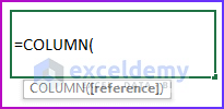
Arguments
| Argument | Required or Optional | Value |
|---|---|---|
| [reference] | Optional | The cell or range of cells for which we want to return the column number. If the reference argument refers to a range of cells, and if the COLUMN function is entered as a horizontal array formula, the COLUMN function returns the column numbers of reference as a horizontal array. |
Return
The function will return the number of a column based on a given cell reference.
How to Use COLUMN Function in Excel: 4 Ideal Examples
In this article, you will see four ideal examples of how to use the COLUMN function in Excel. You will find how to directly use this function and how to combine this function with other Excel functions to get a certain value.
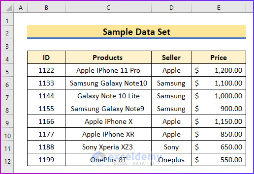
I will use the following sample data set to explain this article.
1. Determine Column Numbers
The basic application or use of the COLUMN function is to find out the column number or numbers of a given cell reference. From the following discussion, you will understand it better.
- Firstly, look at the following image, where you will find the COLUMN function formula with different cell ranges as a reference.
- I will discuss each formula in the following section.

- First, the first formula returns the column number of the current cell. That is 3 for column C.
- Secondly, the following formula will return the G10 cell’s column number, which is 7.
- Thirdly, you will be able to return the column number of the A4:A10 range, which is 1 by using the third function.
- Again, utilizing the fourth function, you can see the column numbers of the A4:F10 dynamic array, which are 1 to 6.
- Lastly, the final formula of the above image returns the first column numbers of the A4:F10 dynamic array, which is 1.
2. Find the First and Last Column Number of Any Range
By using the COLUMN function, you can find the first and last column numbers of any cell range. For that, you have to combine the COLUMN function with the MIN function to find the first column number and the MAX function to see the last column number. See the following steps for a better understanding.
Steps:
- Firstly, to find the first column of a cell range, use the following combination formula in cell D13.
=MIN(COLUMN(C5:E11))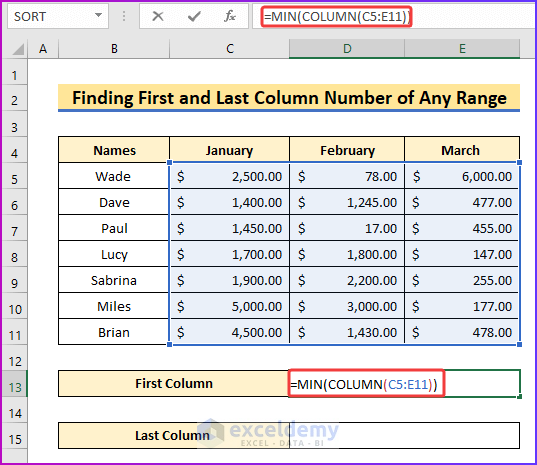
- Secondly, after pressing Enter, you will see the desired column number, which is 3.

- Again, to see the last column number of the same cell range, in cell D15, insert the following combination formula.
=MAX(COLUMN(C5:E11))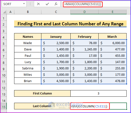
- Finally, after pressing Enter, you can see the number of the last column of this cell range, and it will be 5.

3. Use as Dynamic Column Reference with VLOOKUP Function
In this example, you will see by using the COLUMN function how one can match data with given criteria. To perform this task successfully, you will need the help of the VLOOKUP function of Excel. Now let’s perform this procedure in the following steps.
Steps:
- Firstly, take the following data set, with all the necessary information.
- Along with that, make three extra fields to show the result of this procedure.

- Secondly, to make the formula easier to apply, I will make a dropdown list of the products of column C in cell B15.
- For that, first, choose cell B15 and then go to the Data tab of the ribbon.
- After that, from the Data Tools group, select Data Validation.

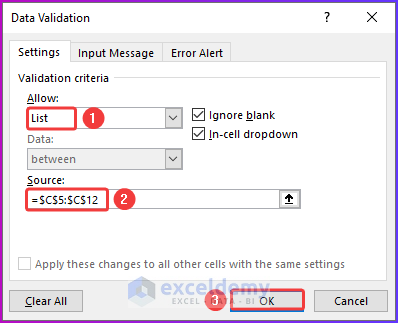
- Thirdly, from the Data Validation dialog box, make the dropdown style List and give the appropriate cell range for creating the dropdown.
- Lastly, press OK.
- So, from the following image, you will be able to see the dropdown containing the product’s name.

- Fifthly, to know the seller name of the particular product of cell B15, use the following combination formula in cell D15.
=VLOOKUP($B15,$C$5:$E$12,COLUMNS($C5:C5)+1,0)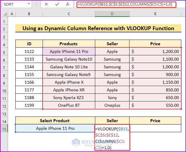
Formula Breakdown
=VLOOKUP($B15,$C$5:$E$12,COLUMNS($C5:C5)+1,0)
- Here, $B14 is the input field. I will enter the input in this field.
- $B$4:$D$11 is the table range where the data is stored.
- COLUMNS($B4:B4)+1 This portion of the formula will return the Seller column values.
- Defining 0 as range_lookup, we are considering the exact match for the comparison.
- Afterward, hit Enter and you will get the desired seller name.

- Moreover, if you also want to find out the price of that product, insert the following formula in cell E15.
=VLOOKUP($B15,$C$5:$E$12,COLUMNS($C5:D5)+1,0)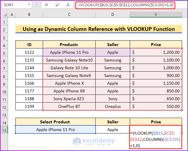
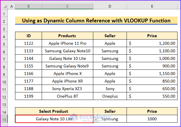
- Finally, press Enter and your job will be done.

- Additionally, by changing the value of cell B15 you can get the result for your desired product.
4. Combine COLUMN Function with MOD and IF Function
Let’s say you have a dataset of the monthly bills of any organization. And you want to increase the bills by a specific number for every third month. You can perform this task by utilizing the IF, COLUMN, and MOD functions together. To do that, see the following steps.
Steps:
- In the beginning, see the following image with the monthly bills, I want to add $500 to every third month’s bill.

- Secondly, in order to do that, write the following formula in cell C5.
=IF(MOD(COLUMN(C7)+1,3)=0,$F$4+C7,C7)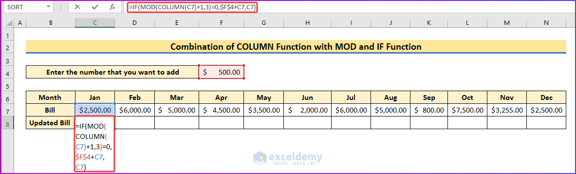
Formula Explanation
=IF(MOD(COLUMN(C7)+1,3)=0,$F$4+C7,C7)
- Here MOD(COLUMN(B4)+1,3) finds every third month from the dataset.
- $E$8+B4 will add the current bill with the input bill if the condition is true.
- B4 is used if the condition is false, it will print the previous bill.
- Thirdly, press Enter and you will find the same result as C5 in D5 as it is the first month.
- In order to see the result for the entire row and all the columns, drag AutoFill to the right.
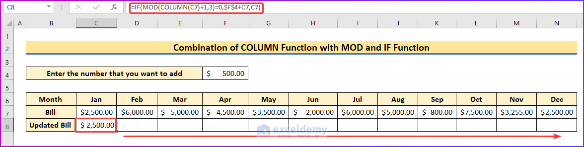
- Finally, you will be able to add $500 with the values of every third month in the following picture.

Things to Remember
- This function will deliver a #NAME! Error if you provide an invalid reference in the argument.
- In the fourth method, I created my data set from the second column. If your data set starts from another column, then you have to modify the formula along with that change
Download Practice Workbook
You can download the free Excel workbook here and practice on your own.
Conclusion
That’s the end of this article. I hope you find this article helpful. After reading the above description, you will be able to understand how to use the COLUMN function in Excel. Please share any further queries or recommendations with us in the comments section below.
Therefore, after commenting, please give us some moments to solve your issues, and we will reply to your queries with the best possible solutions.
<< Go Back to Excel Functions | Learn Excel
Get FREE Advanced Excel Exercises with Solutions!
