Introduction to the MOD Function
- Function Objective:
Returns the remainder after a number is divided by a divisor.
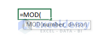
- Syntax:
=MOD(number, divisor)
- Arguments Explanation:
| Argument | Required/Optional | Explanation |
|---|---|---|
| number | Required | Dividend or the number that has to be divided. |
| divisor | Required | Integer number by which you want to divide the dividend. |
- Return Parameter:
The remainder of a division.
Method 1 – Using MOD Function to Find the Remainder
Steps:
➤ In cell D5, type:
=MOD(B5,C5)➤ Press Enter, autofill the rest of the cells in Column D, and you’ll get all the remainder at once.
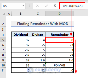
Some facts about the MOD function while determining the remainders should be noted. The remainder will always follow the +/—sign of the divisor, and it doesn’t matter if a dividend is positive or negative.
Another important fact is that if you divide a number with a decimal, the function will return a wrong output. This is illustrated in Row 9, as the value 32 is divisible by 1.6, and the remainder should have been 0, but here, the function has returned the value 1.6. So, this function is useful only with integer divisors, and you cannot expect the function to return an accurate +/—sign.
Method 2 – Determining Odd or Even Numbers with MOD Function
Steps:
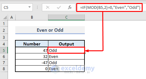
➤ In cell C5, type:
=IF(MOD(B5,2)=0,"Even","Odd")➤ Press Enter and autofill the entire column with Fill Handle.
Method 3 – Performing Calculation on Only Odd Rows with MOD Function
Steps:
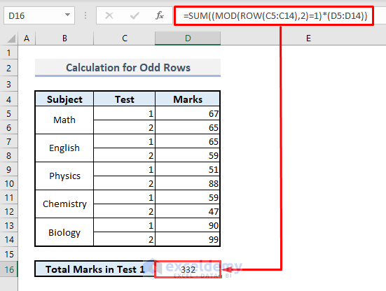
➤ In cell D16, enter the following formula:
=SUM((MOD(ROW(C5:C14),2)=1)*(D5:D14))➤ Press Enter, and the function will return the total marks for all subjects in Test 1.
How Does This Formula Work?
➤ ROW function extracts all the row numbers of the range of cells C5:C14 and will return an array of:
{5;6;7;8;9;10;11;12;13;14}
➤ MOD function finds out only odd-numbered rows from these values and will return:
{TRUE;FALSE;TRUE;FALSE;TRUE;FALSE;TRUE;FALSE;TRUE;FALSE}
➤ Finally, the SUM function sums all the values by following the logical value- TRUE- and ignores another logical value- FALSE.
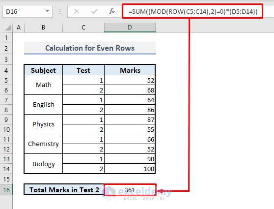
Method 4 – Performing Calculation on Only Even Rows with MOD Function
Steps:
➤ In cell D16, enter the following formula:
=SUM((MOD(ROW(C5:C14),2)=0)*(D5:D14))➤ After pressing Enter, you’ll get the calculated sum for all subjects in Test 2.
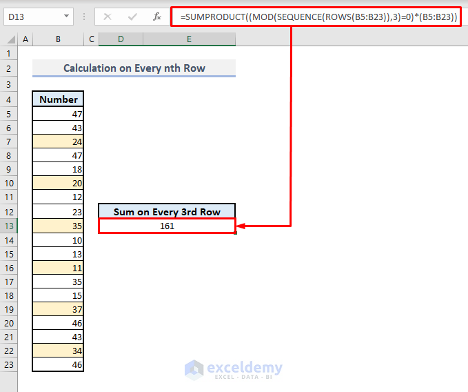
Method 5 – Carrying out Calculation on Every nth Row with MOD Function
Steps:
➤ In cell E13, enter the following formula:
=SUMPRODUCT((MOD(SEQUENCE(ROWS(B5:B23)),3)=0)*(B5:B23))➤ Press Enter, and the resultant value will be shown.
How Does This Formula Work?
➤ Here, the ROWS function returns the total number of rows- 19 from the range of cells B5:B23.
➤ SEQUENCE function returns the serial of 19 numbers starting from 1, and the array will look like this:
{1;2;3;4;5;6;7;8;9;10;11;12;13;14;15;16;17;18;19}
➤ MOD function then divides all these 19 numbers by 3 and returns the logical value TRUE for all divisions where no remainder was found. So, the return values from this step will be:
{FALSE;FALSE;TRUE;FALSE;FALSE;TRUE;FALSE;FALSE;TRUE;FALSE;FALSE;TRUE;FALSE;FALSE;TRUE;FALSE;FALSE;TRUE;FALSE}
➤ Finally, the SUMPRODUCT function extracts data from the specified rows where the logical value TRUE is assigned and then returns the sum of those values.
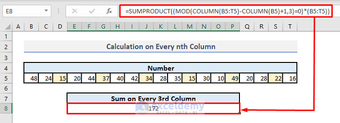
Method 6 – Carrying Out Calculation on Every nth Column with MOD Function
Steps:
➤ In cell E8, enter the following formula:
=SUMPRODUCT((MOD(COLUMN(B5:T5)-COLUMN(B5)+1,3)=0)*(B5:T5))➤ After pressing Enter, you’ll get the resultant value of 172.
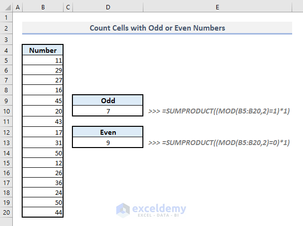
Method 7 – Counting Cells Containing Odd or Even Numbers with SUMPRODUCT and MOD Functions
Steps:
➤ In cell D10, enter the following formula:
=SUMPRODUCT((MOD(B5:B20,2)=1)*1)➤ Press Enter to get the total count of odd numbers in Column B.
➤ Copy the formula, replace 1 with 0 for the MOD function to find the even numbers, and input the modified formula in Cell D13.
➤ Press Enter to get the total count for even numbers.
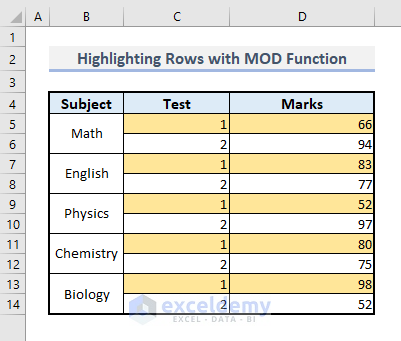
Method 8 – Using the MOD Function to Highlight Cells
Steps:
➤ Select the range of cells C5:D14.
➤ Under the Home tab, select the More Rules command from the Conditional Formatting and Highlight Cell Rules drop-downs in the Styles group of commands.
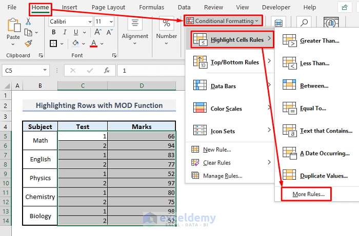
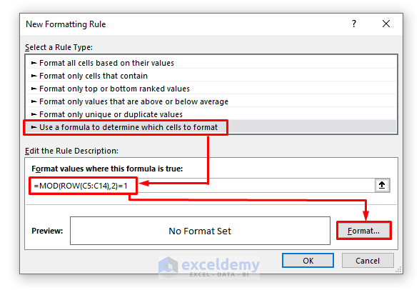
➤ In the New Formatting Rule dialogue box, select “Use a formula to determine which cells to format” from the Rule Type options.
➤ Go to the Rule Description box and type the following formula:
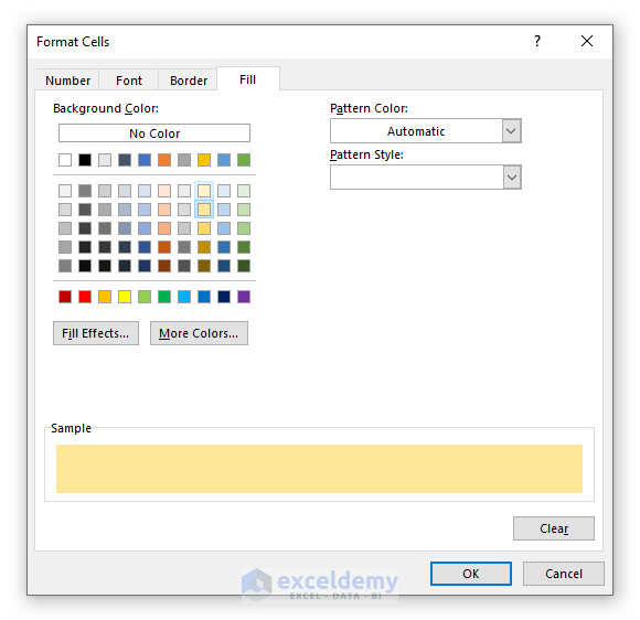
=MOD(ROW(C5:C14),2)=1➤ Press the Format option. Another dialogue box will appear.
➤ From the Fill tab, choose any color you want to highlight the cells
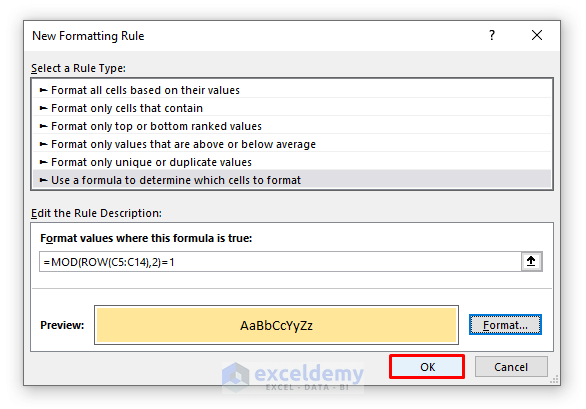
➤ Press OK, and you’ll be brought to the previous dialogue box.
➤ You’ll be shown a preview of the highlighted cell in the New Formatting Rule dialogue box. Press OK.
Like the picture below, you’ll find your highlighted rows with the selected color.
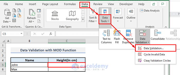
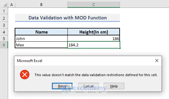
Method 9 – Using Data Validation with MOD Function in Excel
Steps:
➤ Select cell C5.
➤ Under the Data ribbon, choose the Data Validation command from the Data Tools drop-down. A dialogue box named Data Validation will appear.
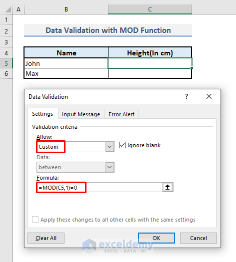
➤ Under the Settings tab, select Custom in the Allow box for Validation criteria.
➤ In the formula box, enter:
=MOD(C5,1)=0➤ Press OK.
➤ Use the Fill Handle from cell C5 to copy the cell format into the next cell C6.
➤ Enter a height in integer value in C5, and you’ll be shown no error message if you’ve just put an integer value.
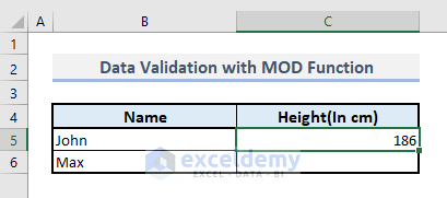
➤ Input a height in decimal value in cell C6, and you’ll be shown an error message.
This is how you can assign a fixed format for a data entry in a certain range of cells.
Read More: [Fixed!] Excel MOD Function Not Working
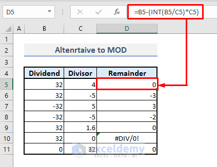
Alternative to the MOD Function to Find the Remainder
Steps:
➤ In cell D5, enter the following formula:
=B5-(INT(B5/C5)*C5)➤ After pressing Enter and auto-filling the entire column with the Fill Handle, you’ll find all the remainder at once.
Things to Keep in Mind
MOD function always returns a similar +/- sign as the divisor.
The divisor must be an integer value in the MOD function. Otherwise, you won’t get the accurate value of the remainder.
If the divisor in the MOD function is 0, the function will return a #DIV/0 error.
Download the Practice Workbook
You can download the Excel workbook and practice.
Excel MOD Function: Knowledge Hub
<< Go Back to Excel Functions | Learn Excel
Get FREE Advanced Excel Exercises with Solutions!
