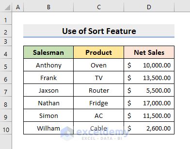
Method 1 – Sort Value in Alphabetical Order in Excel with Sort Featur
STEPS:
- Select the range B5:D10.
- Go to Home ➤ Editing ➤ Sort & Filter ➤ Sort A to Z.
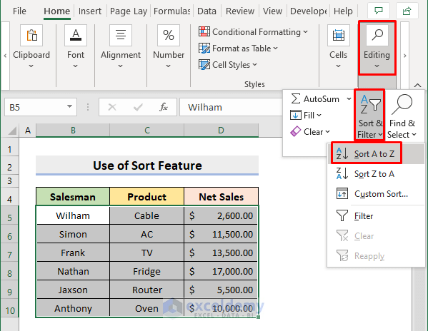
- You’ll get the sorted result.
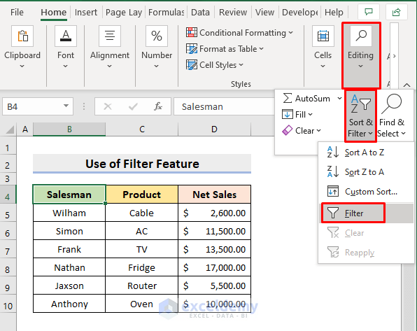
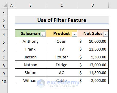
Method 2 – Apply Excel Filter Feature to Set Data in Alphabetical Order
STEPS:
- Click B4.
- Select Home ➤ Editing ➤ Sort & Filter ➤ Filter.
- Press the drop-down beside the Salesman header and select Sort a to Z.
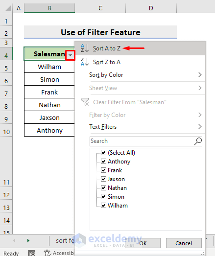
- It’ll return the sorted data.
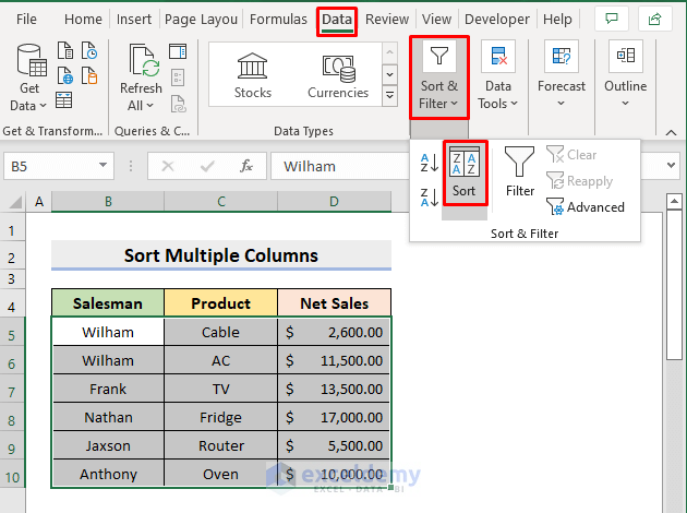
Method 3 – Sort Multiple Columns in Excel
STEPS:
- Select the range B5:D10.
- Select Data ➤ Sort & Filter ➤ Sort.
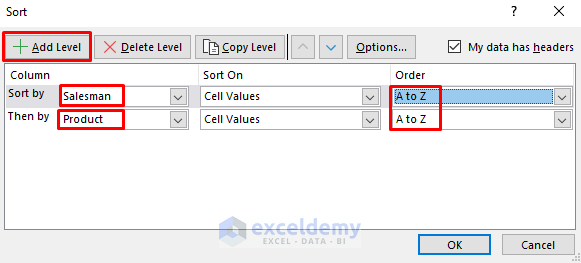
- Sort dialog box will pop out.
- Press Add Level.
- Select Salesman in Sort by and Product in Then by fields.
- Select A to Z from the Order options and press OK.
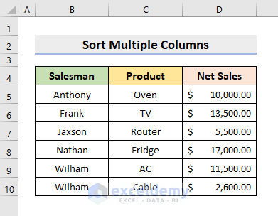
- You’ll get the desired sorted data.
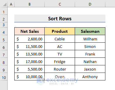
Method 4 – Alphabetically Sorting Rows
STEPS:
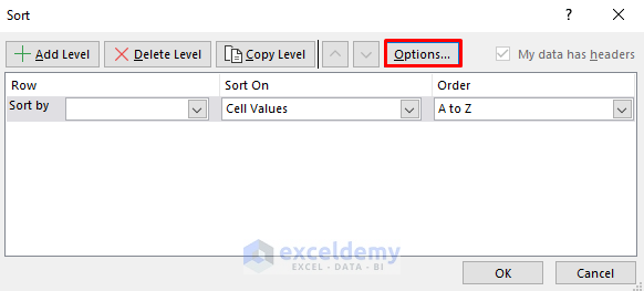
- Select the range and go to Data ➤ Sort & Filter ➤ Sort.
- Sort dialog box will pop out. Press Options.
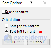
- Select the circle for Sort left to right and press OK.
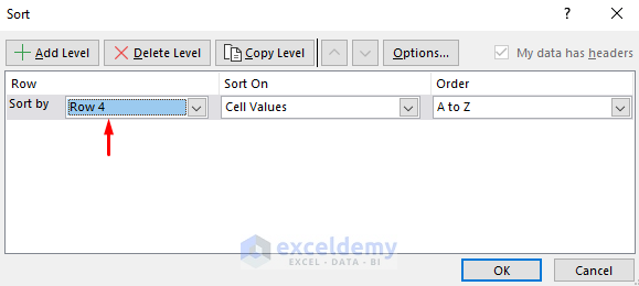
- Select Row 4 (Headers row) and select A to Z in Order.
- Press OK.
- It’ll return the reorganized data.
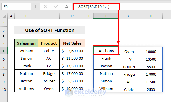
Method 5 – Order Data in Excel Using SORT Function
STEPS:
- Select cell F5 at first.
- Type the formula:
=SORT(B5:D10,1,1)- Press Enter and it’ll spill the rearranged data.
Method 6 – Create a Helper Column for Sorting Value in Alphabetical Order
STEPS:
- Select cell E5 and type the formula:
=COUNTIF($B$5:$B$10,"<="&B5)- Press Enter and use the AutoFill tool to complete the series.
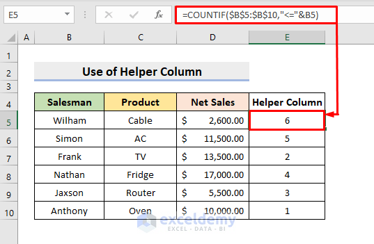
The COUNTIF function compares the text values and returns their relative rank.
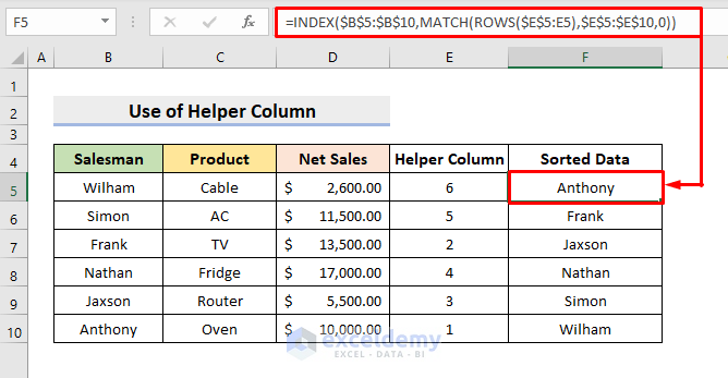
- Select cell F5. Here, type the formula:
=INDEX($B$5:$B$10,MATCH(ROWS($E$5:E5),$E$5:$E$10,0))- Press Enter and complete the rest with the AutoFill tool.
⏩ How Does the Formula Work?
- ROWS($E$5:E5)
The ROW function returns the respective row numbers.
- MATCH(ROWS($E$5:E5),$E$5:$E$10,0)
The MATCH function returns the relative position of the items present in the range $E$5:$E$10.
- INDEX($B$5:$B$10,MATCH(ROWS($E$5:E5),$E$5:$E$10,0))
Finally, the INDEX function returns the value in the row spilled from the MATCH(ROWS($E$5:E5),$E$5:$E$10,0) formula.
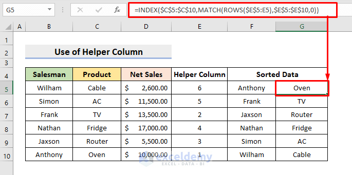
- In cell G5, type the formula:
=INDEX($C$5:$C$10,MATCH(ROWS($E$5:E5),$E$5:$E$10,0))- Press Enter and fill the series using AutoFill.
⏩ How Does the Formula Work?
- ROWS($E$5:E5)
The ROW function returns the respective row numbers.
- MATCH(ROWS($E$5:E5),$E$5:$E$10,0)
The MATCH function returns the relative position of the items present in the range $E$5:$E$10.
- INDEX($C$5:$C$10,MATCH(ROWS($E$5:E5),$E$5:$E$10,0))
Finally, the INDEX function returns the value in the row spilled from the MATCH(ROWS($E$5:E5),$E$5:$E$10,0) formula.
- In cell H5, type the formula:
=INDEX($D$5:$D$10,MATCH(ROWS($E$5:E5),$E$5:$E$10,0))- Press Enter and complete the rest with AutoFill.
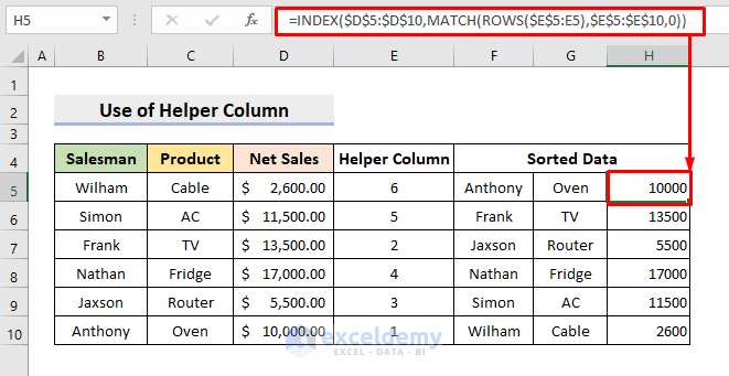
⏩ How Does the Formula Work?
- ROWS($E$5:E5)
The ROW function first returns the respective row numbers.
- MATCH(ROWS($E$5:E5),$E$5:$E$10,0)
The MATCH function returns the relative position of the items present in the range $E$5:$E$10.
- INDEX($D$5:$D$10,MATCH(ROWS($E$5:E5),$E$5:$E$10,0))
Finally, the INDEX function returns the value in the row spilled from the MATCH(ROWS($E$5:E5),$E$5:$E$10,0) formula.
Method 7 – Combine Excel Functions to Organize Data
STEPS:
- Select cell E5 at first.
- Type the formula:
=INDEX($B$5:$B$10,MATCH(ROWS($B$5:B5),COUNTIF($B$5:$B$10,"<="&$B$5:$B$10),0))- Press Enter and use the AutoFill tool to fill the series.
- You’ll get organized data.
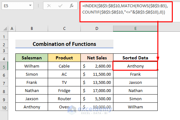
⏩ How Does the Formula Work?
- COUNTIF($B$5:$B$10,”<=”&$B$5:$B$10)
The COUNTIF function compares the text values in the range $B$5:$B$10 and returns their relative rank at first.
- ROWS($B$5:B5)
The ROWS function returns the respective row numbers.
- MATCH(ROWS($B$5:B5),COUNTIF($B$5:$B$10,”<=”&$B$5:$B$10),0)
The MATCH function returns the relative position of the items present in the specified range, which is the output of COUNTIF($B$5:$B$10,”<=”&$B$5:$B$10).
- INDEX($B$5:$B$10,MATCH(ROWS($B$5:B5),COUNTIF($B$5:$B$10,”<=”&$B$5:$B$10),0))
The INDEX function extracts the names in alphabetical order.
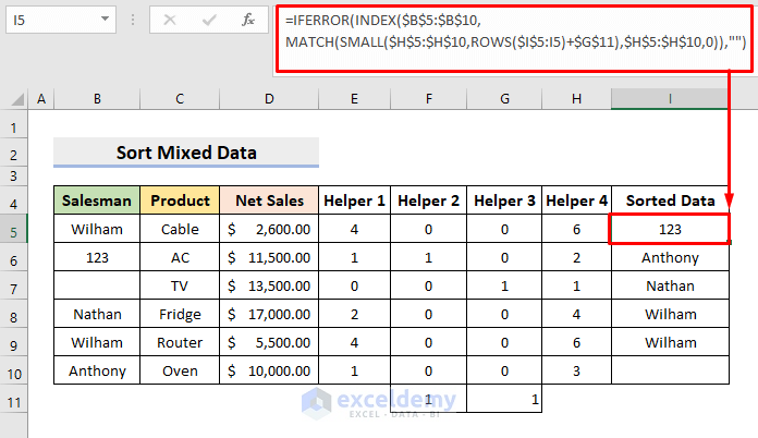
Method 8 – Sort Mixed Data Alphabetically in Excel
STEPS:
- Select cell E5 and type the formula:
=COUNTIF($B$5:$B$10,"<="&B5)- Press Enter and fill the series with AutoFill.
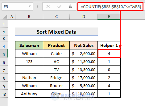
It compares the text values and returns the relative rank.
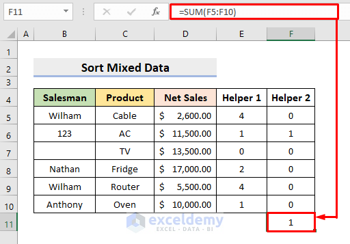
- In cell F5, type the formula:
=--ISNUMBER(B5)- Press Enter and complete the rest with AutoFill.
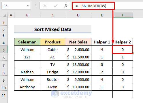
The ISNUMBER function looks for the Number values.
- Select F11 and use the AutoSum feature in Excel to find the total.
- Select cell G5 to type the formula:
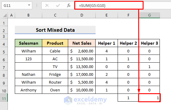
=--ISBLANK(B5)- Press Enter and use AutoFill to complete the rest.
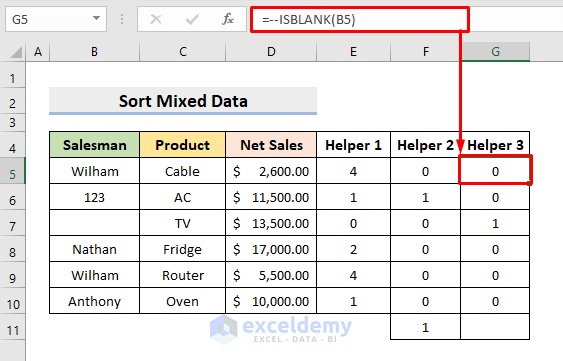
The ISBLANK function looks for the blank cells.
- Select cell G11 and apply the AutoSum feature to find the total.
- Select cell H5 and type the formula:
=IF(ISNUMBER(B5),E5,IF(ISBLANK(B5),E5,E5+$F$11))+$G$11- Press Enter and use the AutoFill tool.
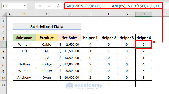
NOTE: This formula with the IF function segregates blanks, numbers, and text values. If the cell is blank, it returns the sum of cell E5 and cell G11. For any numerical value, it returns the comparative rank and adds the total number of blanks. If it is text, it will return the comparative rank and add the total number of numerical values and blanks.
- Select cell I5 and type the formula:
=IFERROR(INDEX($B$5:$B$10,MATCH(SMALL($H$5:$H$10,ROWS($I$5:I5)+$G$11),$H$5:$H$10,0)),"")- Press Enter and use the AutoFill tool.
- It’ll return the sorted data with the blank cell at the last position.
⏩ How Does the Formula Work?
- ROWS($I$5:I5)
The ROWS function returns the respective row numbers.
- SMALL($H$5:$H$10,ROWS($I$5:I5)+$G$11)
The SMALL function returns the specified smallest value from the range $H$5:$H$10.
- MATCH(SMALL($H$5:$H$10,ROWS($I$5:I5)+$G$11),$H$5:$H$10,0)
The MATCH function returns the relative position of the items present in the specified range.
- INDEX($B$5:$B$10,MATCH(SMALL($H$5:$H$10,ROWS($I$5:I5)+$G$11),$H$5:$H$10,0))
The INDEX function extracts the names alphabetically from the range $B$5:$B$10.
- IFERROR(INDEX($B$5:$B$10,MATCH(SMALL($H$5:$H$10,ROWS($I$5:I5)+$G$11),$H$5:$H$10,0)),””)
The IFERROR function returns blank if an error is found, otherwise returns the data.
Problems While Sorting Data in Alphabetical Order in Excel
1. Blank or Hidden Columns and Rows
If there are blank or hidden data, we will not get the sorted result correctly. So, we need to delete the blank cells before applying the Sort operation to ensure a precise result.
2. Unrecognizable Column Headers
Again, if the headers are in the same format as the regular entries, it is likely that they will end up somewhere in the middle of the sorted data. To prevent this, select only the data rows, and then apply the Sort operation.
Download Practice Workbook
Download the following workbook to practice by yourself.
Related Articles
- How to Use Excel Shortcut to Sort Data
- Excel Sort and Ignore Blanks
- How to Sort Data in Excel by Value
- How to Remove Sort in Excel
<< Go Back to Sort in Excel | Learn Excel
Get FREE Advanced Excel Exercises with Solutions!


I have gone through every tip and instruction for Excel issues with sorting alphabetically and I just can’t fix it. I’ve used the TRIM to get rid of extra spaces, I’ve used un-hide rows and columns to be sure there are no hidden rows or columns, I only select the data cells to sort leaving out any column headings or headers, I’ve formatted the columns I’m sorting to be sure they’re in a text format. I just can’t figure it. It’s a simple worksheet but has over 700 rows of data. The program will sort Column E properly but Column C sorts alphabetically at first, then starts over in the middle of the sort on Column E.
Hello Laura,
Sorry to hear your issue. Here, I am suggesting some troubleshooting steps to resolve the problem. But I will encourage you to submit your Excel file in our ExcelDemy Forum so that we can inspect it thoroughly.
1. Remove Non-Printable Characters:
Use =CLEAN(C2) to clean the data.
2. Check for Merged Cells:
Ensure there are no merged cells in your dataset.
Data Consistency:
3. Make sure all data in Column C are of the same type (text).
4. Sort by Multiple Columns:
Use Data > Sort,
and add levels to sort by Column C first and then Column E.
5. Manual Inspection:
Check the middle section where the sort restarts for any anomalies.
6. New Worksheet:
Copy and paste the data into a new worksheet and try sorting again.
Regards
ExcelDemy