Excel Sort and Ignore Blanks (4 Ways)

By default, when we sort data in Excel, it leaves all the blank rows at the end. But we don’t always want this. Sometimes we need to ignore the blanks while applying the sort in Excel. In this article, you will learn 4 ways to sort & ignore blanks in Excel with ease.

How to Sort & Ignore Blanks in Excel (4 Easy Ways)

Look at the following data table. It has blank rows at numbers 7,9 and 11 positions.

Before applying the sorting command, you need to hide them first.

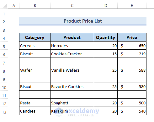
1. Hide Blank Rows to Sort & Ignore Blanks in Excel

To ignore the blank rows while sorting, hiding the blanks is a good option.

To hide all the blanks manually,

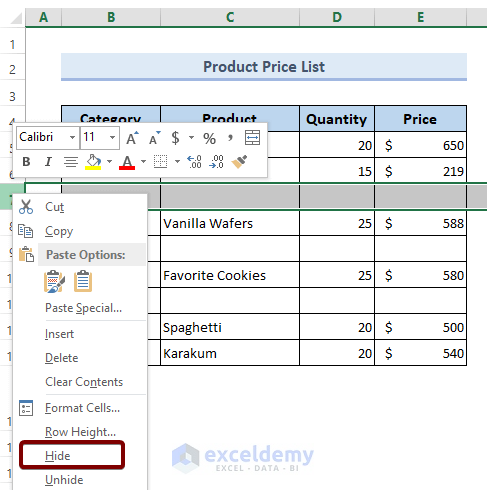
❶ Select the entire row first. Click on any cell of the blank row. Then press the SHIFT + SPACE keys together. This will select the entire row at once.

❷ Right-click on the selection area.

❸ Then click on Hide from the list.

❹ Now select the whole data table.

❺ Go to the Data tab from the main ribbon.

❻ Then click on the A to Z icon to apply the sorting command.

This command will sort the data in ascending order.

❼ Now unhide all the hidden rows. To do that first, right-click on the area in between cells 6 and 8. This is where the first hidden cell resides.

❽ After that select Unhide from the pop-up list.

❾ Continue this process to unhide all the hidden blanks of the data table.

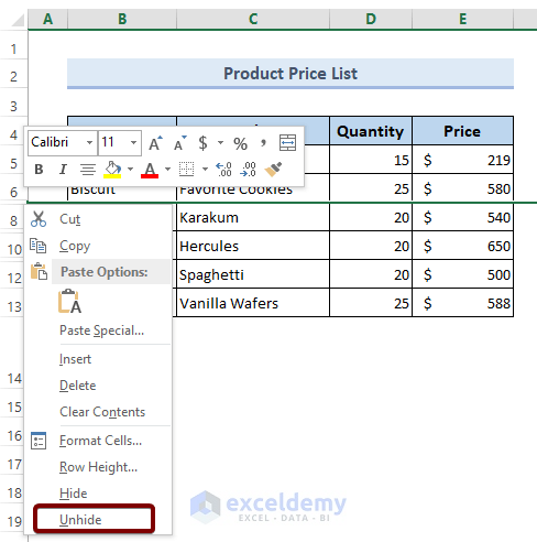
When you are done with all the blank rows unhide, you will see your data is sorted ignoring the blanks like the image below:

Read More: How to Add Sort Button in Excel

2. Use Go To Special to Sort and Ignore Blanks in Excel

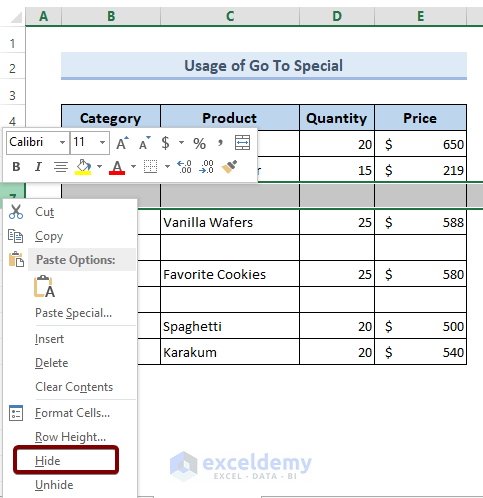
You can use the Go To Special feature to select all the blanks in your data table. Based on your blank row selection, you can hide them all and apply the sorting command.

To do that follow the steps below.

❶ First of all, select the entire data table and go to the Home tab from the main ribbon.

❷ Then go to the Editing group.

❸ Under the Find & Select group, you will find the Go To Special option. Just click on it.

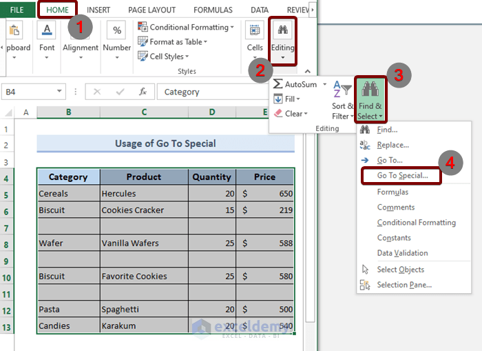
❹ Then the Go To Special dialog box will appear. Select Blanks and hit the OK button.

After that, you will get all the blanks selected. To hide them all,

❺ Right-click on the selection area and then choose Hide from the pop-up list.

So you have all the blank rows hidden. Now apply the sorting command to your data. To do that,

❻ Select the entire data table. Then go to the Data tab. Under the Sort & Filter group, you will find the A to Z icon. Just click on it.

This will sort out your data in ascending order.

❼ Again select the entire data table. Right-click on it and choose Unhide to reveal all the hidden blank rows.

So you will have all the sorted data ignoring the blanks as in the image below.

Read More: How to Use Excel Shortcut to Sort Data

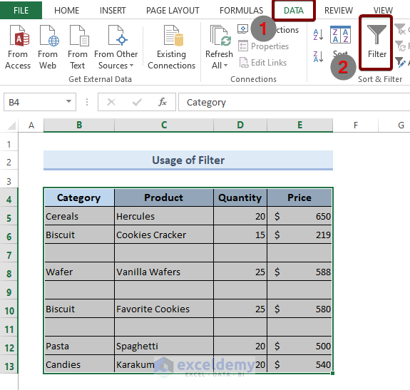
3. Use Filter to Sort and Ignore Blanks in Excel

You can the Filter feature to sort and ignore blanks in Excel.
To do that,
❶ Select the whole data table.
❷ Go to the Data tab. Choose Filter from the Sort & Filter group.

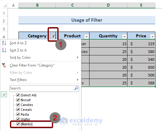
❸ Click on the drop-down icon from the table headers. Uncheck the Blanks and hit OK.

❸ Again select the whole data table. Go to the Data tab and click on the A to Z icon to sort in ascending order.

❹ After that click on the Filter icon from one of the table headers.
❺ Mark check on the Blanks this time and hit OK.

Following the above steps, you will have your data sorted by ignoring the blanks.

Read More: How to Sort Data by Value in Excel

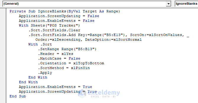
4. Use VBA Code to Sort and Ignore Blanks in Excel

You can use VBA code to sort and ignore the blank rows in Excel.

To do that,

❶ Press ALT + F11 to open the VBA editor.

❷ Then go to Insert > Module to create a new module.

❸ Copy the following code and paste it to the VBA editor.

Private Sub IgnoreBlanks(ByVal Target As Range)
Application.ScreenUpdating = False
Application.EnableEvents = False
With Sheets("POS Tracker")
.Sort.SortFields.Clear
.Sort.SortFields.Add Key:=Range("B5:E13"), SortOn:=xlSortOnValues, _
Order:=xlDescending, DataOption:=xlSortNormal
With .Sort
.SetRange Range("B5:B13")
.Header = xlYes
.MatchCase = False
.Orientation = xlTopToBottom
.SortMethod = xlPinYin
.Apply
End With
End With
Application.EnableEvents = True
Application.ScreenUpdating = True
End Sub

❹ Press CTRL + S to save the VBA code.

❺ Now hit the Run Sub button or press F5 to run the above code.

When the VBA code runs, it will sort data and ignore the blanks as in the picture below:

Read More: How to Undo Sort in Excel

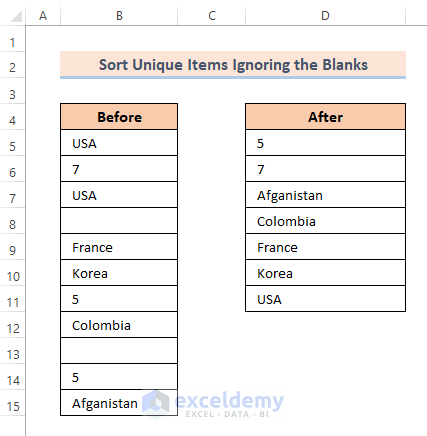
Sort and Ignore Blanks in Excel Keeping the Unique Items Only

In this section, I’m going to show you how to sort data in ascending order ignoring the blanks. If you have blank rows, this method will delete them all. Besides, if you have duplicate values, this method will extract only the unique values and sort them accordingly.

In the following image, under the Before column, we have raw data with duplicate values as well as blanks. In the After column, we will extract only unique values sorted in ascending order ignoring the blank rows.

To do that,

❶ Select cell D5 and insert the following array formula:

❷ After that hold CTRL and SHIFT buttons.

❸ Then press the ENTER button. This will execute the array formula.

❹ Then drag the Fill Handle icon from cell D5 to D11.

Formula Breakdown:

• COUNTIF($D$4:D4,$B$5:$B$15)=0 returns the count value of the cells, where there is a match between $D$4:D4 and $B$5:$B$15.
• ISNUMBER($B$5:$B$15) returns turn if the value in the cell is a number.
• COUNTIF($D$4:D4,$B$5:$B$15)=0)*ISNUMBER($B$5:$B$15) returns either true or false based on the logical multiplication of the COUNTIF($D$4:D4,$B$5:$B$15)=0 and ISNUMBER($B$5:$B$15).
• IF((COUNTIF($D$4:D4,$B$5:$B$15)=0)*ISNUMBER($B$5:$B$15),$B$5:$B$15,”A”),1) returns A if the logical expression becomes false.
• SMALL(IF((COUNTIF($D$4:D4,$B$5:$B$15)=0)*ISNUMBER($B$5:$B$15),$B$5:$B$15,”A”),1) returns the smallest number in the range B5 to B15.
• COUNTIF($B$5:$B$15,”<“&$B$5:$B$15) returns either TRUE or FALSE based on the comparison result between the content of $B$5 and successive cells up to $B$15.
• ISTEXT($B$5:$B$15) evaluates whether the cell range $B$5:$B$15 contains any text item.
• IF(ISTEXT($B$5:$B$15),COUNTIF($B$5:$B$15,”<“&$B$5:$B$15),””),0) returns null string if there’s a text from $B$5 to $B$15. If there’s any number then returns the smallest number.
• SMALL(IF(ISTEXT($B$5:$B$15)*(COUNTIF(D4:$D$4,$B$5:$B$15)=0),COUNTIF($B$5:$B$15,”<“&$B$5:$B$15),””),1),IF(ISTEXT($B$5:$B$15),COUNTIF($B$5:$B$15,”<“&$B$5:$B$15),””),0) returns the smallest to largest number first in the range B5 to B15. After the end of the numbers, it returns the texts in ascending order.

Sort Data and Extract Unique Values Ignoring Blanks in Excel with a Condition

We have a list of products and their availability is marked with either TRUE or FALSE. We want to get a list of sorted items in ascending order based on the filtering result.

Our main target is to extract all the unique items out of the raw data in ascending order with a condition. To do that,

❶ First of all, select the data table.

❷ Go to the Data tab in the main ribbon.

❸ From the Sort & Filter group choose Filter to apply Filter on the data table.

❹ Then insert the following formula in cell F7.

❺ Now hold the CTRL and SHIFT buttons together.

❻ After that hit the ENTER button to execute the array formula.

Now I’ve input TRUE in the Fact box and the following result came along.

If I input FALSE in the Fact box then the Sorted Data column will look like this:

Formula Breakdown:

• COUNTIF($F$6:F6,Table1[Items])=0 returns a count value if there’s a match in between the contents of the Sorted Data column and Items column of the raw data table.
• ISBLANK(Table1[Items]) evaluates whether the Items column contains any blank cell.
• IF(Table1[Fact]=$F$4 processes the input item of the Fact box.
• SMALL(IF(Table1[Fact]=$F$4,IF(ISBLANK(Table1[Items]),””,IF(COUNTIF($F$6:F6,Table1[Items])=0 picks up the smallest item in the Items column.
• MATCH(SMALL(IF(Table1[Fact]=$F$4,IF(ISBLANK(Table1[Items]),””,IF(COUNTIF($F$6:F6,Table1[Items]) looks for a match between the content inserted into the Fact box and the contents of the Items column.
• INDEX(Table1[Items],MATCH(SMALL(IF(Table1[Fact]=$F$4,IF(ISBLANK(Table1[Items]),””,IF(COUNTIF($F$6:F6,Table1[Items]) returns the index number of the cell of the Items column if there’s a match in between the item of the Fact box and that of the Items column.
• ISNUMBER(Table1[Items]) checks whether the item in the Items column is a number or not.

Things to Remember

• You can use CTRL + SHIFT + L to apply the filter.
• Press F5 to run an Excel VBA code.
• To execute an array formula, press CTRL + SHIFT + ENTER.

Download Practice Workbook

You can download the Excel file from the following link and practice along with it.

Conclusion

To sum up, we have discussed 4 ways to sort and ignore blanks in Excel. You are recommended to download the practice workbook attached along with this article and practice all the methods with that. And don’t hesitate to ask any questions in the comment section below. We will try to respond to all the relevant queries. And please visit our website Exceldemy to explore more.

Related Articles

• How to Sort Data in Excel Using Formula
• How to Sort Data in Alphabetical Order in Excel
• How to Sort Alphanumeric Data in Excel
• How to Sort by Color in Excel
• How to Remove Sort by Color in Excel
• How to Remove Sort in Excel

<< Go Back to Sort in Excel | Learn Excel