How to Sort Data Using a Formula in Excel – 2 Methods

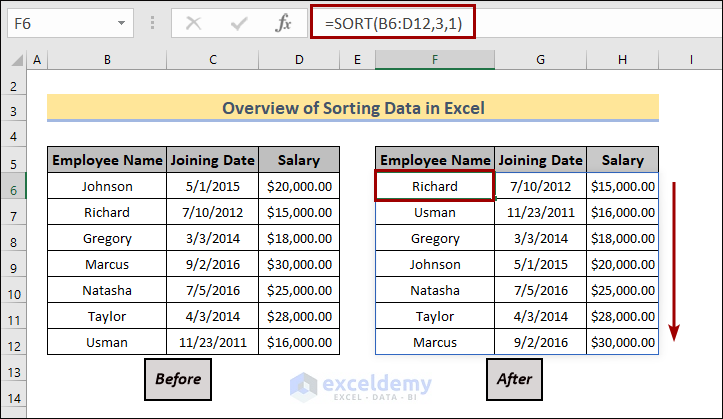
This is an overview:

Method 1 –Using the SORT Function

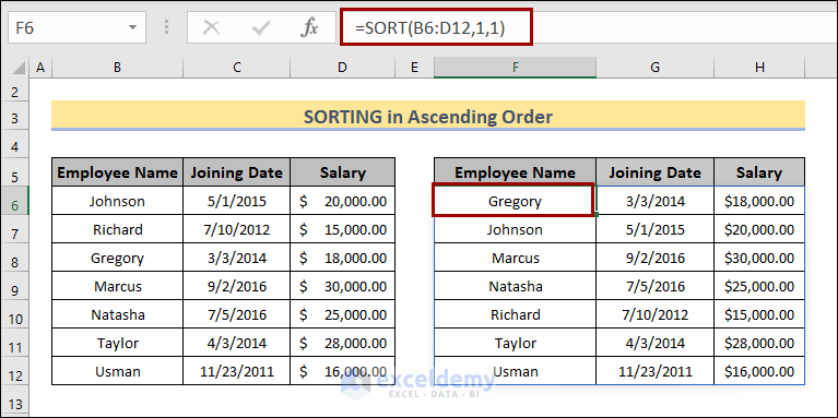
1.1 Sorting in Ascending Order

• Select a blank cell.
• Enter the formula: =SORT(B6:D12,1,1)
  

Text values in the first column are sorted in ascending order.

To sort the third column that contains number values, change the sort_index or the 2nd argument in the formula:

• Select a blank cell
• Use the formula: =SORT(B6:D12,3,1)

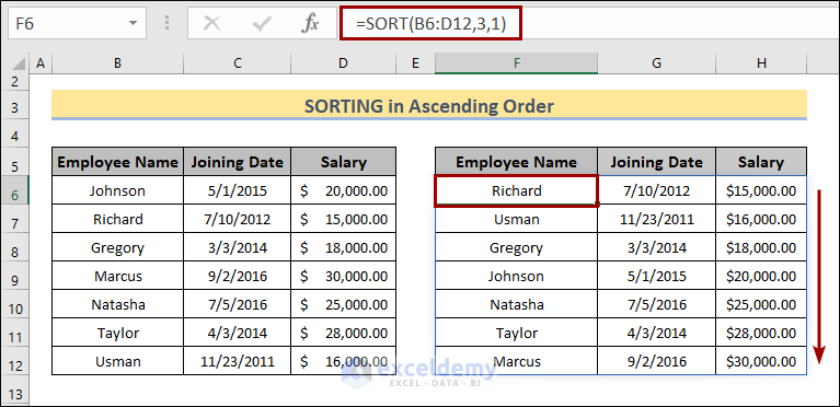
Note: After sorting, the date column will be displayed in General format. Change the format to Date.

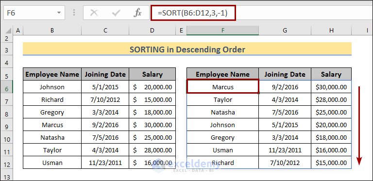
1.2 Sorting in Descending Order

• Select a blank cell.
• Enter the formula: =SORT(B6:D12,3,-1)
  

The third column is sorted in descending order.

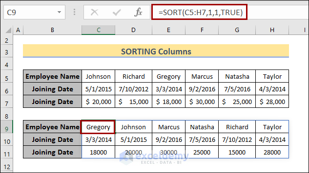
1.3 Sorting Rows

• Select a cell.
• Enter the formula: =SORT(C5:H7,1,1,TRUE)
  

Data is sorted horizontally in alphabetical order: A-Z.

Method 2 – Using the INDEX, MATCH and COUNTIF Functions

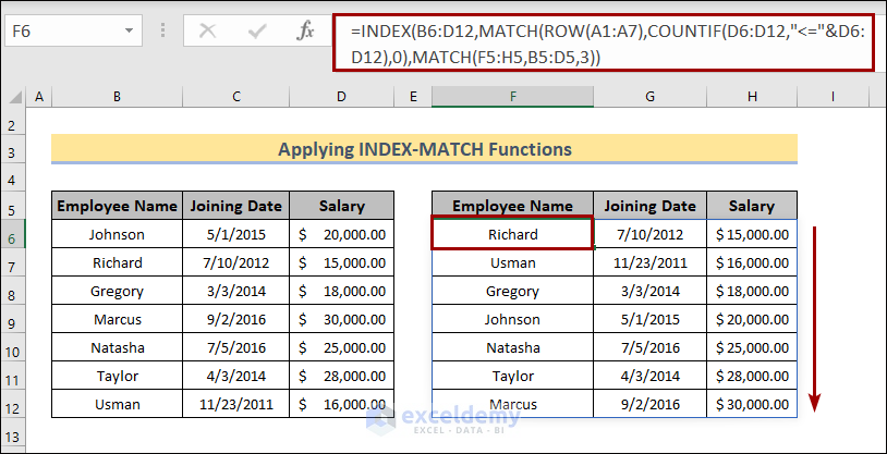
2.1 Ascending Order

• Select a cell.
• Use the following formula and press Enter:
  =INDEX(B6:D12,MATCH(ROW(A1:A7),COUNTIF(D6:D12,”<=”&D6:D12),0),MATCH(F5:H5,B5:D5,3))

Data in the third column is sorted in ascending order.

2.2 Descending Order

• Select a cell.
• Use the following formula:
  =INDEX(B6:D12,MATCH(ROW(A1:A7),COUNTIF(D6:D12,”>=”&D6:D12),0),MATCH(F5:H5,B5:D5,3))

Data in the third column is sorted in descending order.

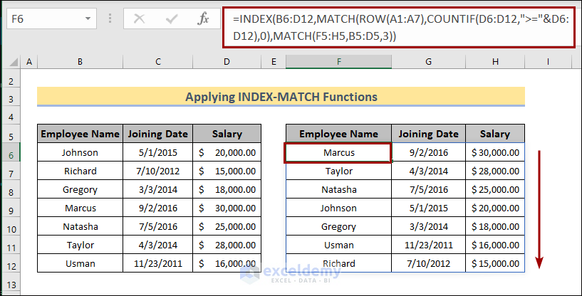
Note: This is an Array Formula. Press Ctrl + Shift + Enter for older Excel versions.

Download Practice Workbook

Download the practice workbook.

Frequently Asked Questions

How do I automatically sort data in Excel?

To sort data automatically:

• Select a range.
• Go to the Data tab > Sort & Filter > Sort A to Z.

Can I create custom sorting orders using formulas?

Yes, use the SORT function, the MATCH and SEQUENCE functions to define a custom sorting order.

How do I sort data in a table automatically?

Click the column header and choose “Sort Ascending” or “Sort Descending.”