How to Add Sort Button in Excel (7 Methods)

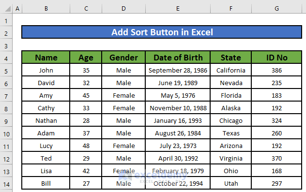
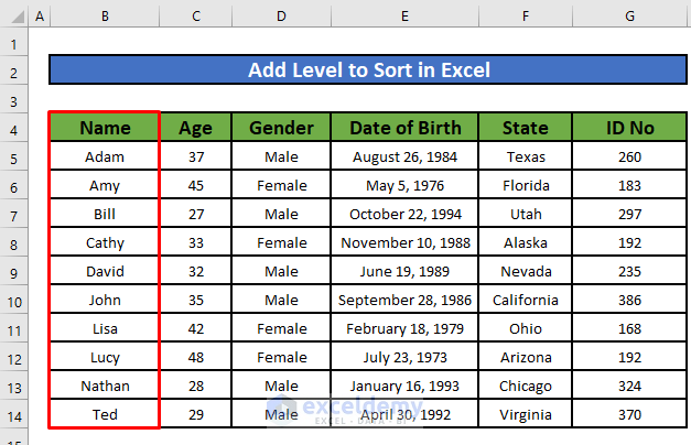
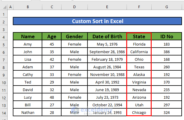
We have an Excel file that contains information about the employees of a company. The worksheet has the Name, Age, Gender, Date of Birth, States they come from, and their ID No. We will add a sort button to sort the information of the employees in several ways.

Method 1 – Add Level in Sort Option to Sort in Excel

Steps:

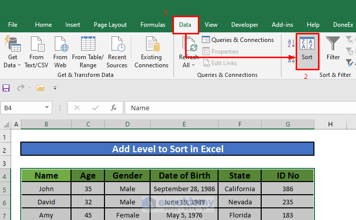
• Select all the cells in the data range including the column headers.
• Go to the Data tab and select the Sort option from the Sort & Filter group.

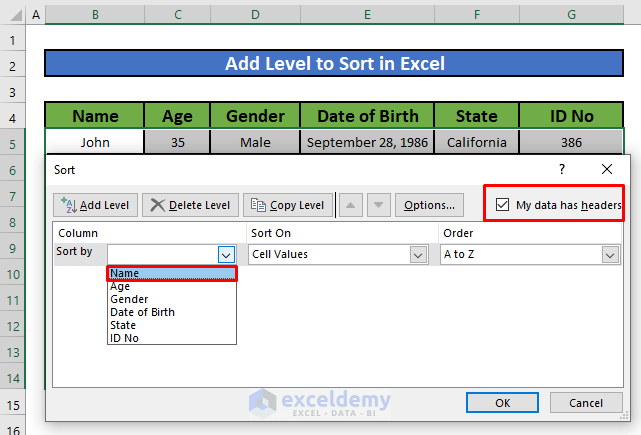
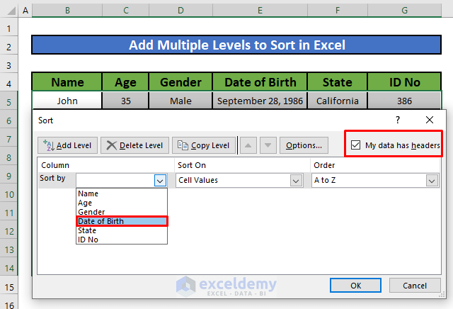
• A new window titled Sort will appear. Check the box for My data has headers.
• Click on the Sort by drop-down menu and select the Name column.

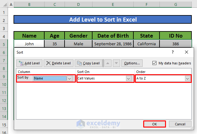
• The default values are cell values for the Sort On drop-down and A to Z for the order. Leave these in. We are sorting the values or names of the employees in the Name column and we will sort them in alphabetical order.
• Click on OK.

• We will see that all the employee names in the Name column have been sorted in alphabetically ascending order.

We can also add multiple levels to sort the data.

• Take a fresh copy of the worksheet or delete the existing level by clicking on Delete Level just beside the Add Level.
• Check the box for My data has headers.
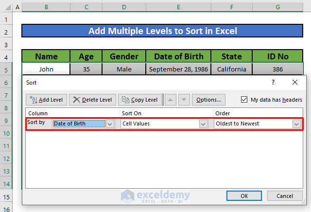
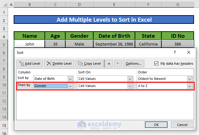
• Select the Date of Birth from the Sort by drop-down menu.

• The Date of Birth column is our first level in sorting. So, our rows will be first sorted by the Date of Birth of the employees. Then, it will be sorted based on the next levels. The order of sorting for this column will be Oldest to Newest.

• Click on the Add Level button again to add the second level for sorting.

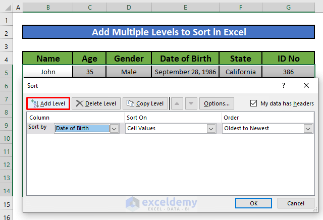
• Select the Gender column from the Then by drop-down menu.

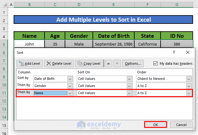
• Click on Add again and enter Name as the third level to sort the data.
• Click OK to sort the rows.

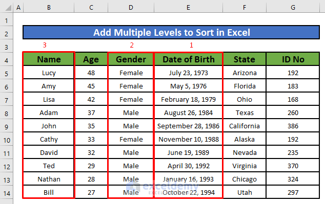
• All of the rows in our data range have been sorted by Date of Birth first, then by Gender, and finally by the Names of the employees.

Read More: How to Undo Sort in Excel

Method 2 – Create a Custom Sort List in Excel

Steps:

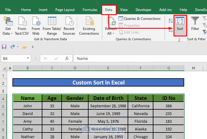
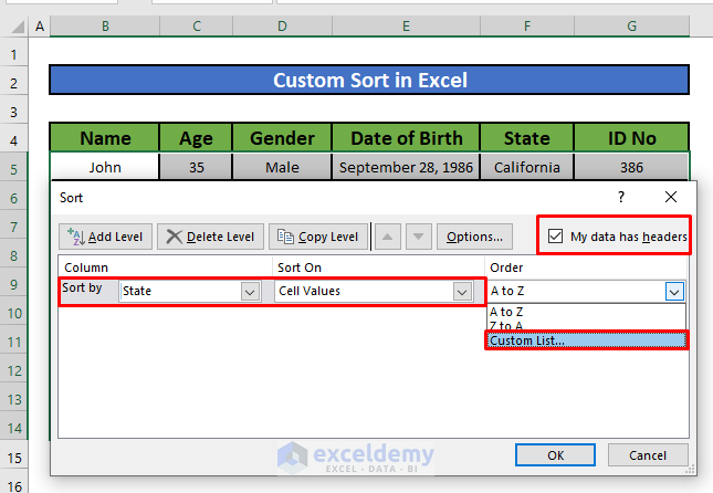
• Select all the cells in our data range including the column headers.
• Go to the Data tab and select the Sort option from the Sort & Filter group.

• Select the State column from the Sort by drop-down menu.
• Click on the Order drop-down and select Custom List.

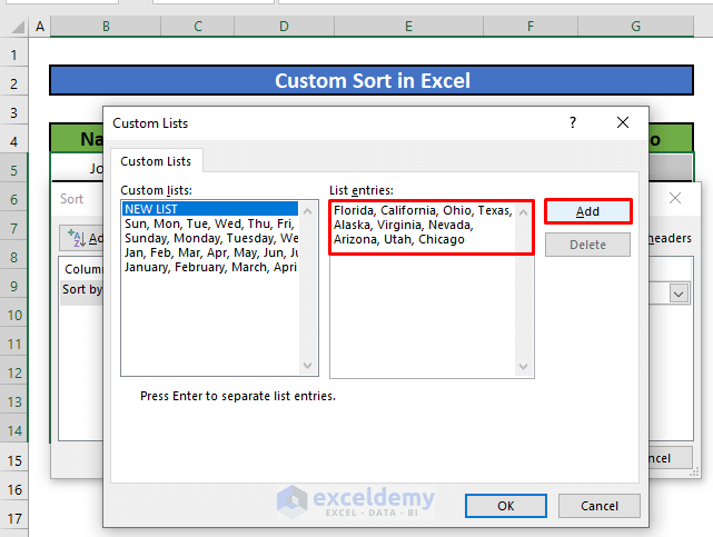
• Enter the list of states separated by a comma(,). This list will be used to sort the rows based on the States.
• Click on OK.

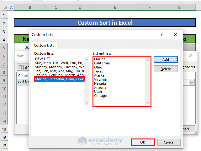
• A list of states has been created.
• Click on the OK button to confirm the list.

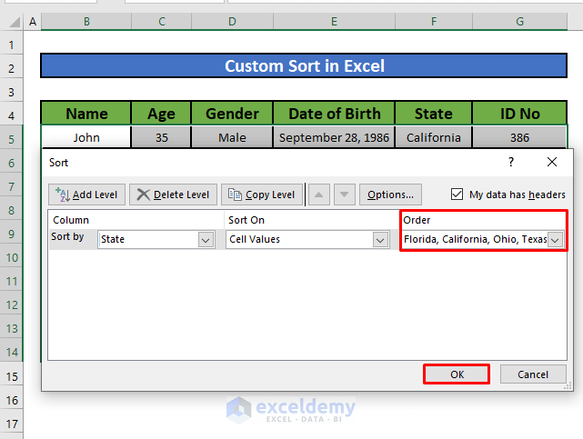
• The Order drop-down has an additional option containing the list we have just created. Select the list if it is not selected.
• Click on OK.

• All the rows of the data range have been sorted based on the list of states we have created.

Read More: How to Use Excel Shortcut to Sort Data

Method 3 – Sort the Data Using the Filter Option

Steps:

• Select all the cells in the data range including the column headers.
• Go to the Data tab and select the Filter option from Sort & Filter.

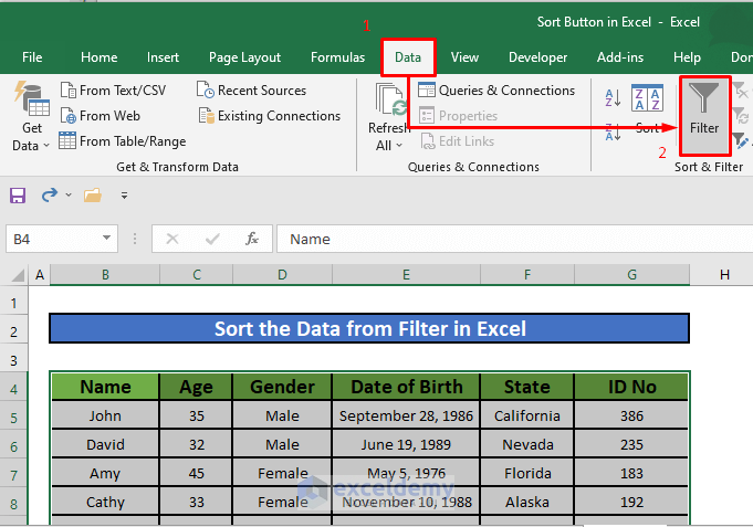
• You’ll get a small downward arrow on the down-right corner of each column header.
• Click on the arrow for the Age column. A new window will appear.
• Select the Sort Smallest to Largest option from that window.

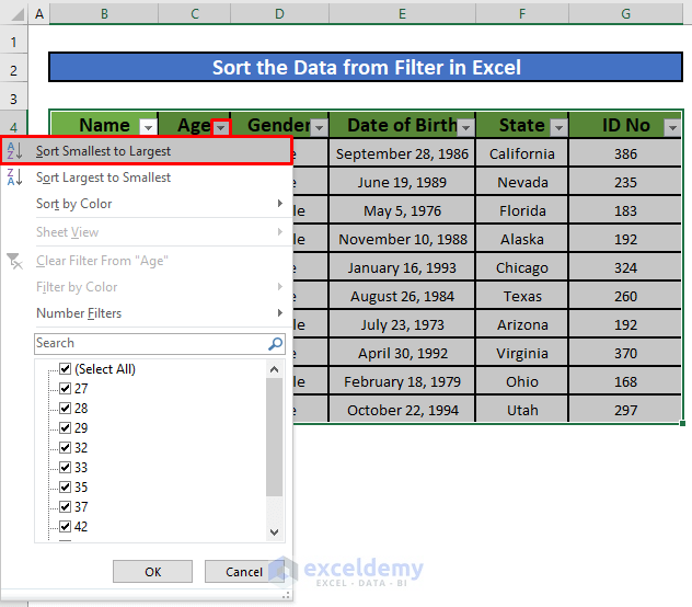
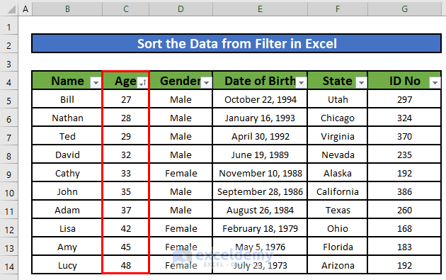
• Rows in the Age column are sorted in ascending order from lowest to greatest.

Read More: How to Sort by Color in Excel

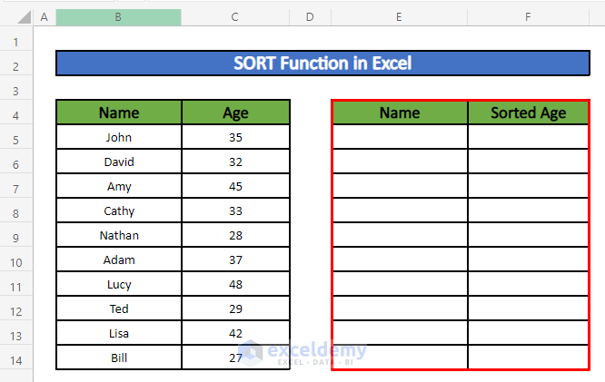
Method 4 – Sort the Data with the SORT Function in Excel 365

Steps:

• Create two columns with column headers Name and Sorted Age like below.

• Use the below formula in cell E5.

• The SORT function takes 3 arguments.
  • B5:C14 is the cell range we want to sort.
  • 2 indicates the second column or the Age column in the range.
  • -1 means we want to sort the data in descending order.

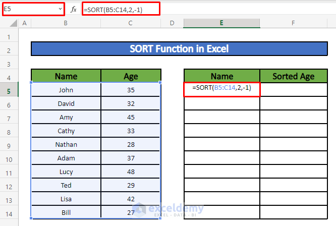
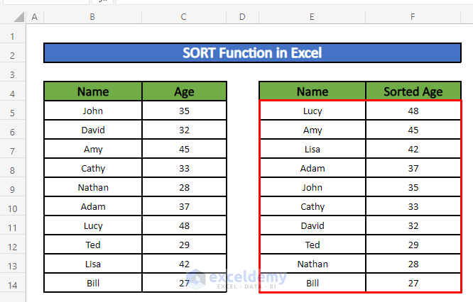
• Hit Enter.

Read More: How to Sort Data in Excel Using Formula 

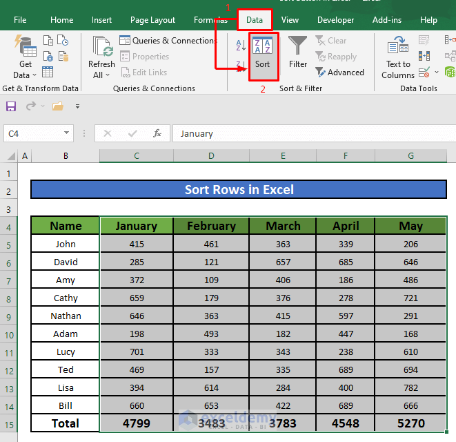
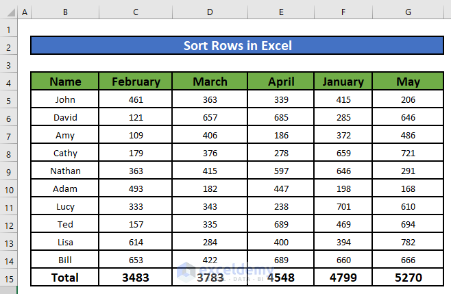
Method 5 – Sort the Data in a Row

Suppose we have the sales volumes of each month from January to May for every employee. We will sort the rows to reorder the total sales volume in ascending order.

Steps:

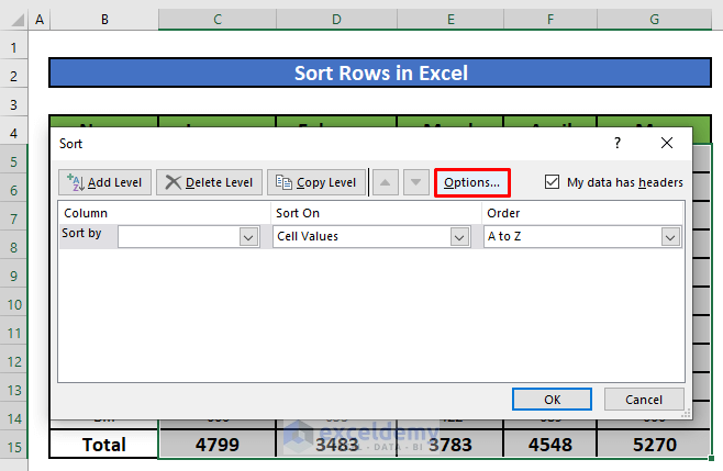
• Select all the cells in the data range except the Name column.
• Go to the Data tab and select the Filter option from Sort & Filter.

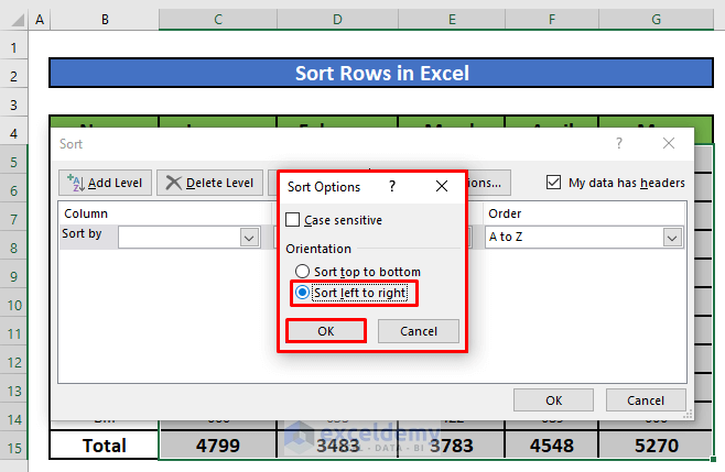
• Select Options from Sort.

• A new window titled Sort Options will appear. Select Sort left to right from there.
• Click OK.

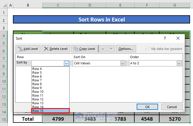
• If we now click on the Sort by drop-down menu, we will see that it is not showing column titles anymore. It now shows Rows. But the rows do not have any title but numbers like Row 4, Row 5, etc.
• Select Row 15.

• Click OK.

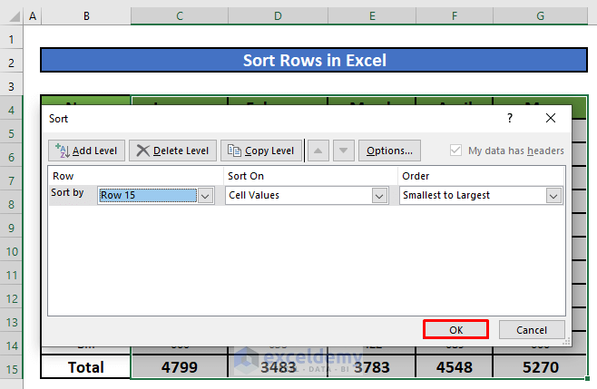
• Here’s the result.

Read More: How to Remove Sort by Color in Excel

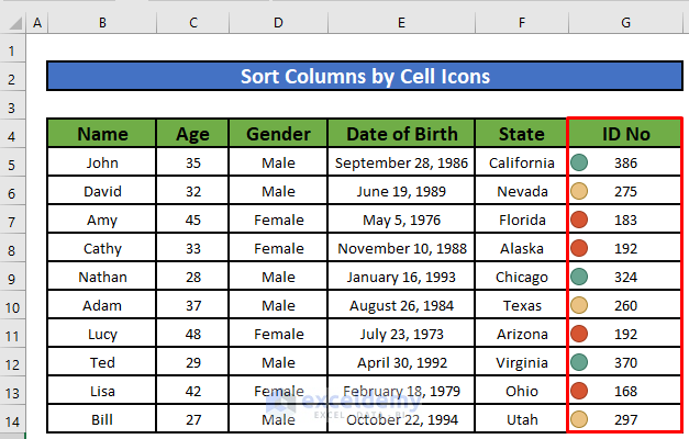
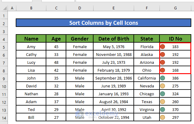
Method 6 – Sort the Data in Column by Cell Icons

We will sort the rows based on the ID No column.

Steps:

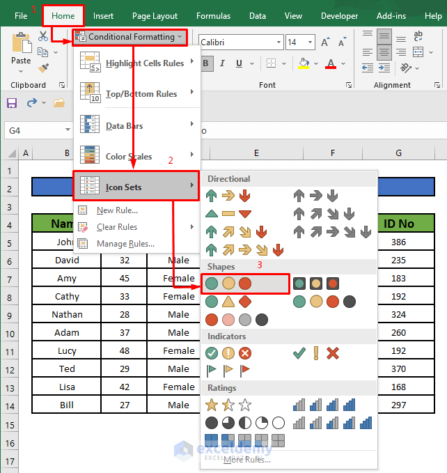
• Select Conditional Formatting from the Styles section under the Home tab.
• A drop-down menu will appear. Select Icon Sets from that list.
• Another list with different sets of shapes will appear. Select a set of shapes like the image below.

• The cells in the ID No column now have different types of shapes besides their values based on the range of values.

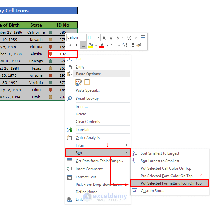
• Click on a cell with a red circle and right-click.
• Select Sort from that window.
• Another list will appear which has different options to sort the data. Select the Put Selected Formatting Icon On Top option from that list.

• All the cells with the red circle shapes are now on the top of the column.

Read More: How to Sort Data by Value in Excel

Method 7 – Add a Sort Button to the Quick Access Toolbar in Excel

Steps:

• Go to the Data tab and right-click on Sort.  A window will appear.
• Click on Add to Quick Access Toolbar from that window.

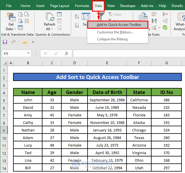
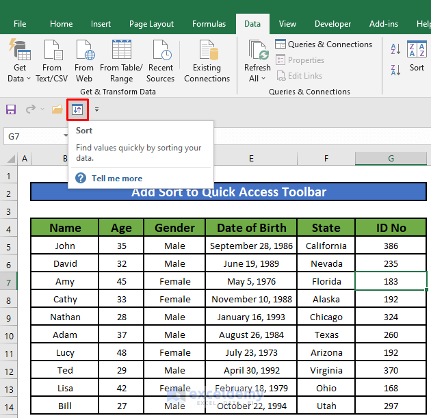
• Sort is added to the Quick Access Toolbar.

Related Content: How to Remove Sort in Excel 

Things to Remember

• You will need Excel 365 to use the SORT function.
• You should always check the My Data has headers option except for sorting the rows. This option will be disabled when sorting the rows.

Download the Practice Workbook

Related Articles

• How to Sort in Ascending Order in Excel
• How to Sort Alphanumeric Data in Excel
• Excel Sort and Ignore Blanks

<< Go Back to Sort in Excel | Learn Excel