In this article, we will discuss Excel’s ISBLANK function, as in the following gif.
Excel ISBLANK Function: Syntax and Argument
ISBLANK Function (Quick View)
![]()
Summary:
Excel ISBLANK function takes a cell reference, evaluates if the cell is blank, then returns TRUE or FALSE accordingly. The function is available from Excel 2007 onwards.
- Generic Syntax
=ISBLANK(value)- Argument Description
| Argument | Requirement | Explanation |
|---|---|---|
| value | Required | The cell to be evaluated. |
Return Value:
Returns a Boolean value (TRUE or FALSE): TRUE if the cell is blank, FALSE otherwise.
ISBLANK Function in Excel: 3 Suitable Examples
In this article, we will illustrate 3 handy examples of the usage of the Excel ISBLANK function. Firstly, we will use the function with conditional formatting. Secondly, we will filter values using the function. Finally, we will use the function to find the value of the first non-empty cell of a dataset.
Example 1 – ISBLANK Function with Condition
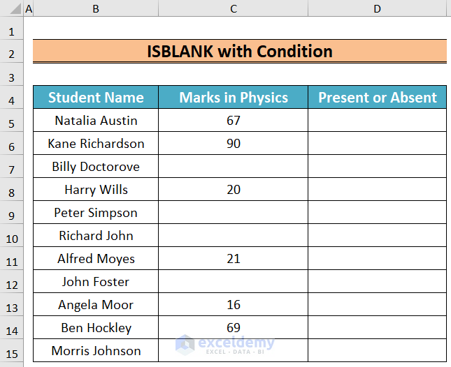
In this example, we will apply a condition to a dataset by using the ISBLANK function combined with the IF function. In the dataset below, we have the names of some students and their marks in Physics. Using the ISBLANK function, we will determine whether each student was Present or Absent in the examination.
Steps:
- In cell D5, enter the following formula:
=IF(ISBLANK(C5),"Absent","Present")- Press Enter.
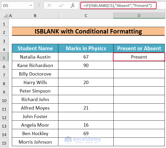
The result (whether the student was present or not) is returned.
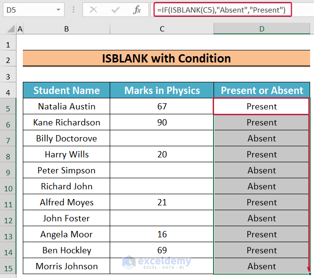
- Drag the Fill Handle down to Autofill the rest of the cells below.
Formula Breakdown:
- ISBLANK(C5): returns TRUE if cell C4 is blank, and FALSE if it is not.
- IF(ISBLANK(C6),”Absent”,”Present”): returns “Absent” if TRUE, and “Present” if FALSE.
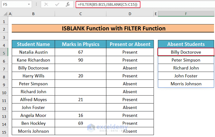
Example 2 – ISBLANK Function with FILTER Function
Now we will make a list of the absent students combining the ISBLANK function with the FILTER function.
Steps:
- In cell F5 enter the following formula:
=FILTER(B5:B15,ISBLANK(C5:C15))- Press Enter.
As a result, we have a list of students who were absent.
Formula Breakdown:
- ISBLANK(C5:C15): returns an array of TRUE or FALSE values; TRUE for a number and FALSE for a blank cell in the range C4 to C20.
- FILTER(B5:B15,ISBLANK(C5:C15)): returns the corresponding name in the range B4 to B20 for a TRUE.
Example 3 – Finding the First Non-Blank Cell Value Using ISBLANK Function
To find the first non-blank cell value in a range, we will combine the ISBLANK function with the INDEX and MATCH functions.
Steps:
- In cell F5 enter the following formula:
=INDEX(C5:C15,MATCH(FALSE,ISBLANK(C5:C15),0))- Press Enter.
The first non-blank value of the dataset is returned.
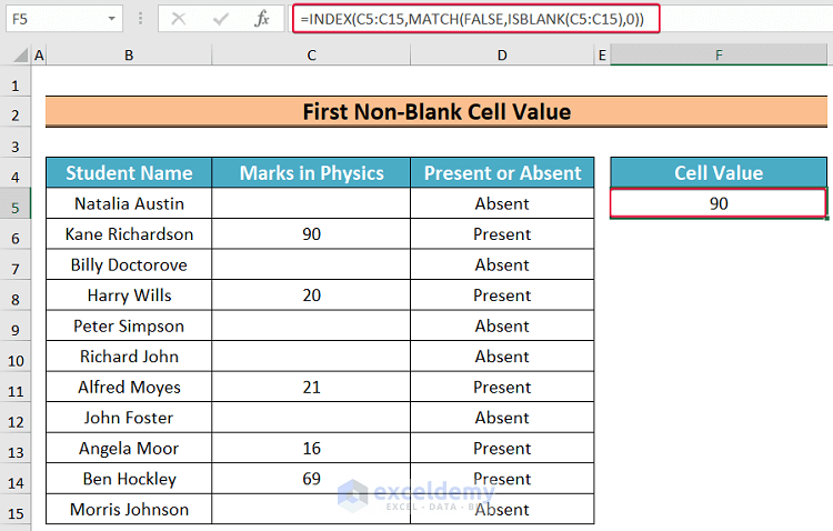
- ISBLANK(C5:C15): Returns an array of TRUE and FALSE values for the C5:C15 range. If the formula finds any blank cell in the range, it will return TRUE otherwise FALSE.
- MATCH(FALSE,ISBLANK(C5:C15),0): The MATCH function looks for a lookup value within an array and returns its relative position. Here, the function looks for FALSE in the array returned by the ISBLANK function. The 0 (zero) means it will return the position of the first value that exactly matches with FALSE in the ISBLANK(C5:C15) array. In this case, the result will be 2, since the ISBLANK function returns a FALSE value in the second position in the array.
- INDEX(C5:C15,MATCH(FALSE,ISBLANK(C5:C15),0)): The INDEX function takes the index of a value within an array and returns the value. Here, the index function takes 2 from the MATCH(FALSE,ISBLANK(C5:C15),0) expression as input, and looks for the 2nd value in the C5:C15 range. It returns 90.
Read More: How to Use ISBLANK Function to Check If Cell Is Blank
Excel ISBLANK Function: Knowledge Hub
- Excel ISBLANK vs IsEmpty
- How to Use Excel ISBLANK to Identify Blanks in Range
- How to Use ISBLANK Function in Excel for Multiple Cells
- How to Use ISBLANK Function for Conditional Formatting in Excel
- How to Use SUMIF and ISBLANK to Sum for Blank Cells in Excel
<< Go Back to Excel Functions | Learn Excel
Get FREE Advanced Excel Exercises with Solutions!
