In a large dataset with numerous entries, there may be many blank cells. You may need to identify those empty cells. We can use the ISBLANK function to find blank cells in our dataset and conditional formatting to highlight them.
How to Use the ISBLANK Function for Conditional Formatting in Excel: 3 Suitable Methods
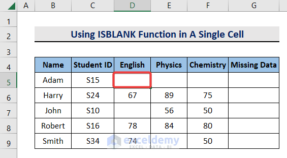
Method 1 – Using the ISBLANK Function for Conditional Formatting in a Single Cell
Steps:
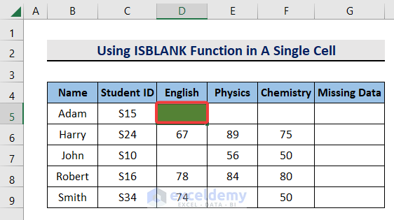
- Select the cell where you want to apply the function. We are selecting the blank cell D5.
- Select the Home tab.

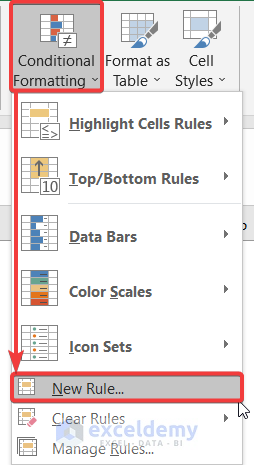
- Go to Conditional Formatting and choose New Rule.
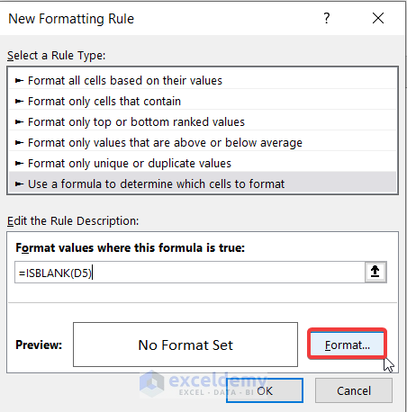
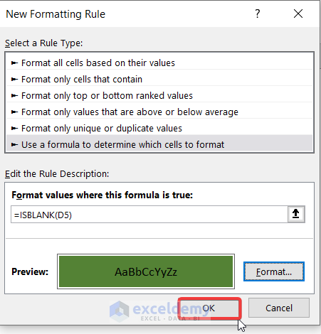
- From the New Formatting Rule dialog box, click on Use a formula to determine which cells to format.

- Use the following formula in the formula box:
=ISBLANK(D5)- Click on Format.
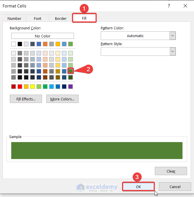
- You will get different options to highlight the cell. If you want to fill the cell with any specific color, click on Fill, then select any color of your choice.
- Click OK.

- The New Formatting Rule dialog box will appear again. Click OK to apply the formatting to the selected cell.
- Here’s the result. The cell is blank so it got filled with color.
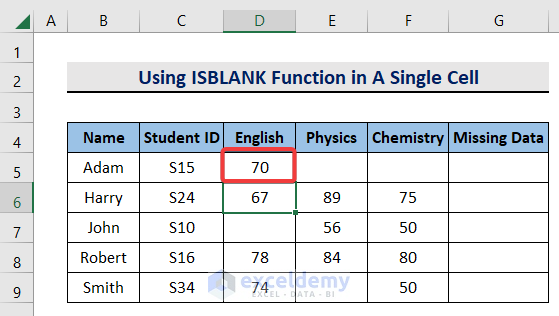
- If you put any value into the cell and press the Enter key, the cell will lose its formatting.
Read More: How to Use SUMIF and ISBLANK to Sum for Blank Cells in Excel
Method 2 – Applying the ISBLANK Function for Conditional Formatting in Multiple Cells
Case 2.1 – Using the Manage Rules Command for Conditional Formatting
Steps:
- Follow Method 1 to highlight a single cell with the ISBLANK function.
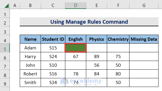
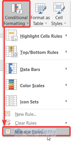
- Go to Conditional Formatting and click on Manage Rules.
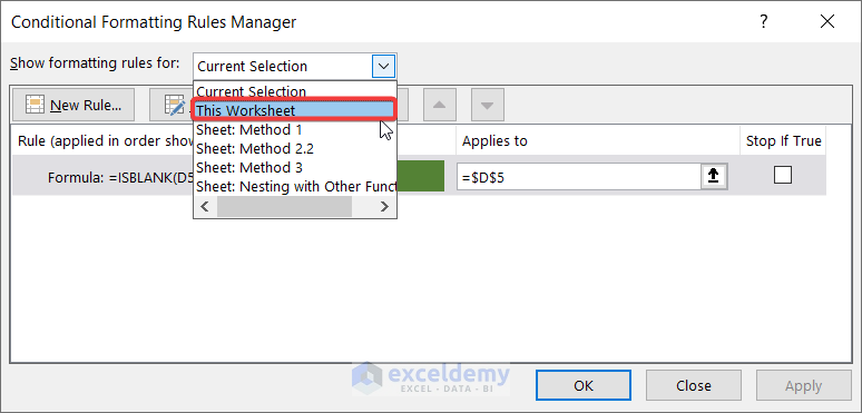
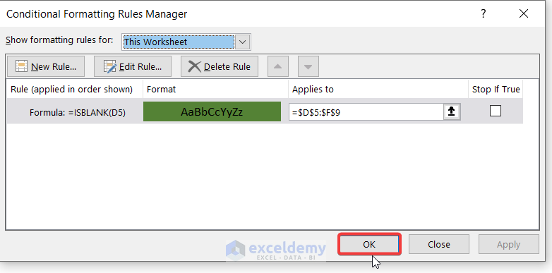
- From the menu bar, select This Worksheet.
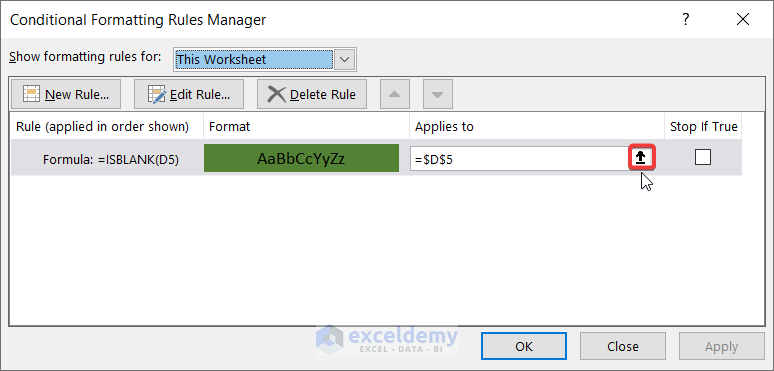
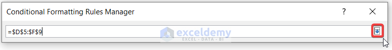
- Select the up-arrow sign next to the range bar for the rule already in place.
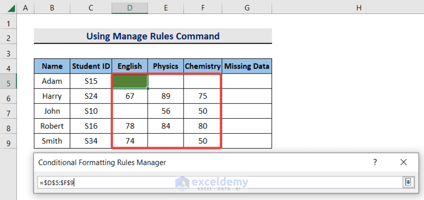
- Select the new range where you want the rule to apply, such as cells D5:F9.
- Click on the down arrow sign at the end of the range bar.
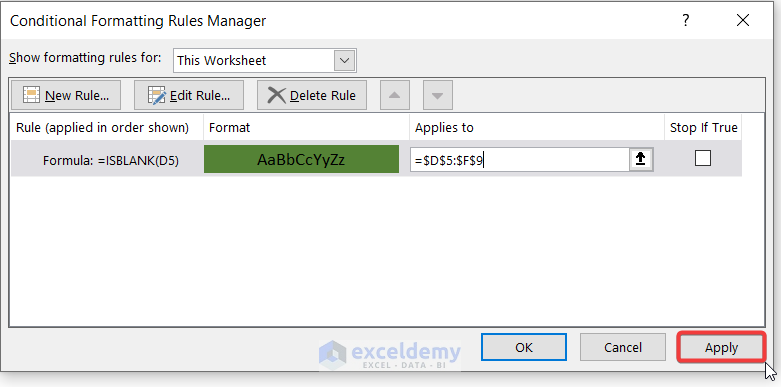
- Click on Apply.
- Press OK.
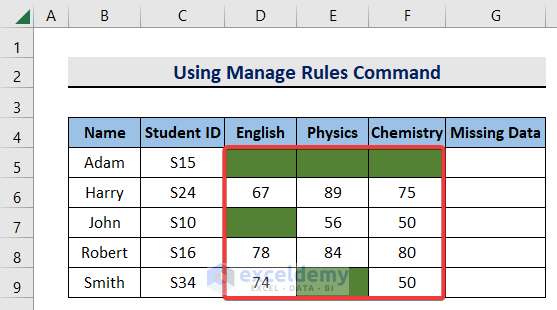
- All the empty cells in the specified range will be filled with your chosen color.
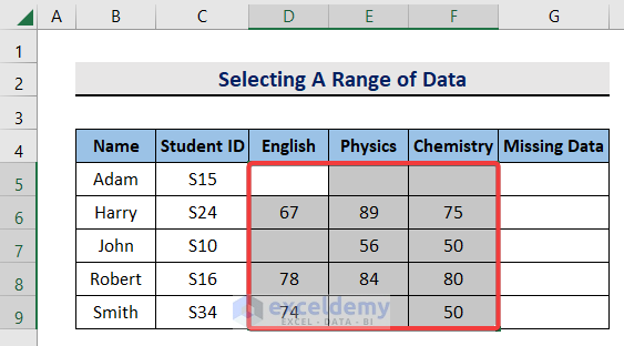
Case 2.2 – Selecting a Range of Data
Steps:
- Select the range of cells where you want to apply the function. We are selecting cells D5:F9.
- Select the Home tab.

- Go to Conditional Formatting and open New Rule.

- From the New Formatting Rule dialog box, click on Use a formula to determine which cells to format.

- Use the following formula in the formula box.
=ISBLANK(D5:F9)- Click on Format.
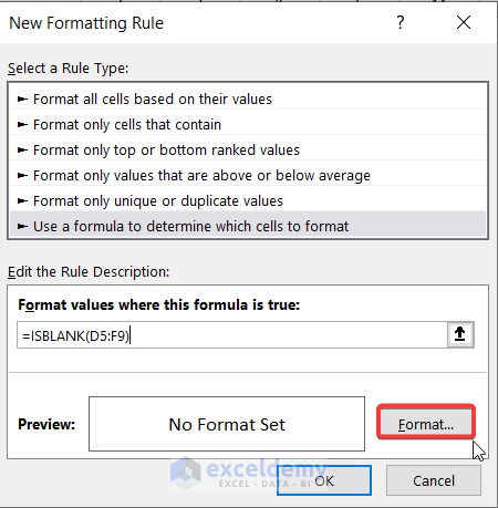
- Choose your highlighting color or pattern in the Fill tab and click OK.

- The New Formatting Rule dialog box will appear again. Click on OK.

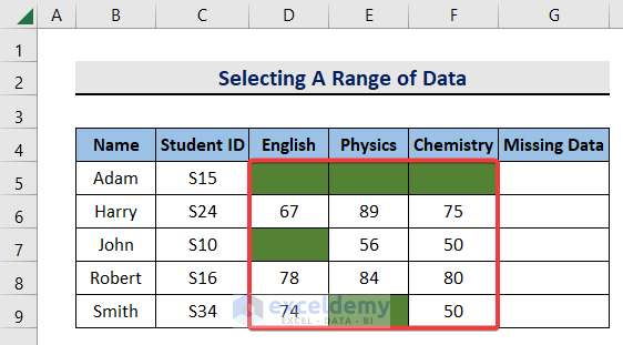
- Here are the results.
Read More: How to Use ISBLANK Function to Check If Cell Is Blank in Excel
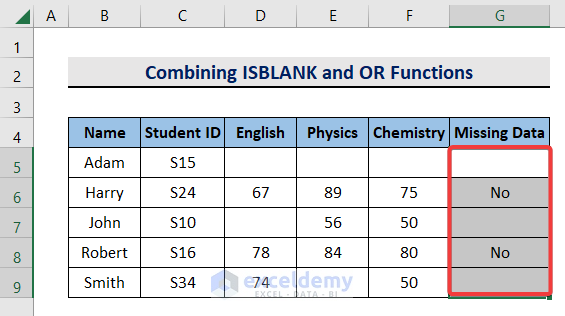
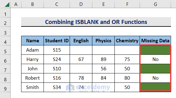
Method 3 – Combining ISBLANK and OR Functions for Conditional Formatting in Excel
In the data set, there are students who have not received their grades in all subjects. If there is even one empty cell in any of the fields (English, Physics, and Chemistry), the oversight is noted in Missing Data. We’ll use the column to display a blank value if at least one of the scores is missing, then highlight those cells.
Steps:
- Select the range where you want to apply Conditional Formatting. We are selecting G5:G9.
- Select the Home tab.

- Go to Conditional Formatting and select New Rule.

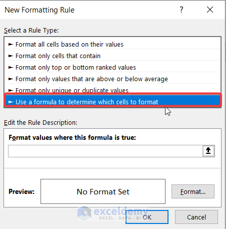
- From the New Formatting Rule dialog box, click on Use a formula to determine which cells to format.
- Use the following formula into the formula box:
=OR(ISBLANK(D5),ISBLANK(E5),ISBLANK(F5))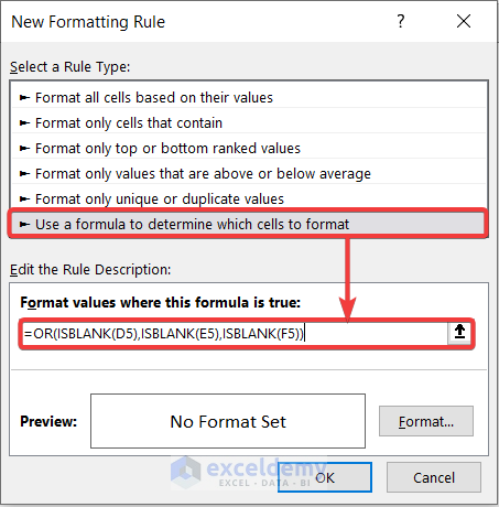
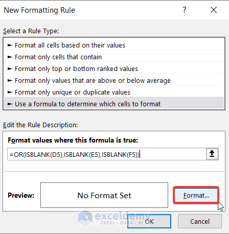
- Press Format.
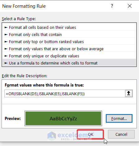
- Click on Fill, select any color of your choice, and press OK.

- The dialog box will appear again. Click on OK.
- If any data is missing in the subject fields, the corresponding cell in the Missing Data field will turn into your chosen color.
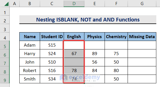
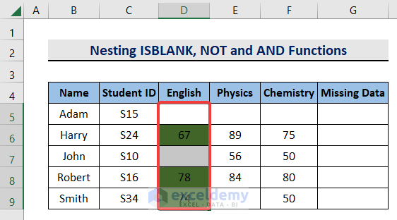
Nesting ISBLANK, NOT, and AND Functions to Ignore Blank Cells with Conditional Formatting
Steps:
- Select the range where you want to apply Conditional Formatting. We put D5:D9.
- Select the Home tab.

- Go to Conditional Formatting and select New Rule.

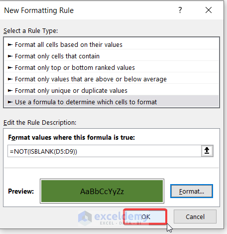
- In the New Formatting Rule dialog box, click on Use a formula to determine which cells to format.

- Use the following formula in the formula box:
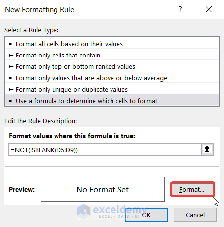
=NOT(ISBLANK(D5:D9))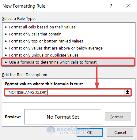
- Press Format.
- Click on Fill and select any color of your choice, then press OK.
- The dialog box will appear again. Click on OK.
- You will see that the non-empty cells will be highlighted.
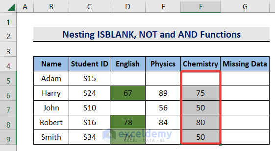
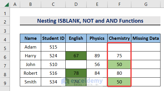
We can also highlight cells with specific criteria and ignore empty cells from the range. Let’s highlight those values that are lower than 75 from column F. If we were to only check the value of the cell, blank cells would be implicitly converted to 0 and highlighted. We can use the NOT and ISBLANK functions to get around that.
Steps:
- Select the range where you want to apply Conditional Formatting. We are selecting F5:F9.
- Select the Home tab.
- Go to Conditional Formatting and choose New Rule.

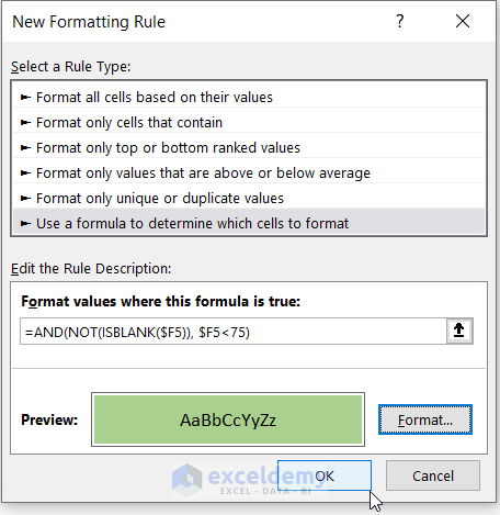
- In the New Formatting Rule dialog box, click on Use a formula to determine which cells to format.

- Insert the following formula into the formula box:
=AND(NOT(ISBLANK($F5)), $F5<75)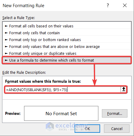
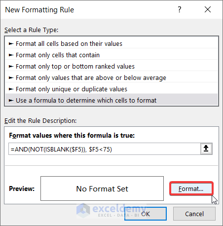
- Press Format.
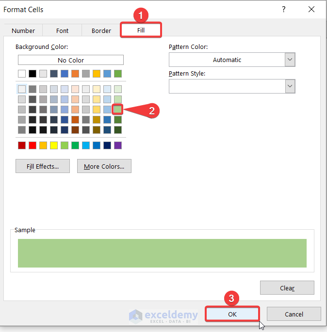
- Click on Fill and select any color of your choice, then press OK.
- The Formatting dialog box will appear again. Click on OK.
- Here are the results.
Download the Practice Workbook
Related Articles
- How to Use ISBLANK Function in Excel for Multiple Cells
- How to Use Excel ISBLANK to Identify Blanks in Range
- Excel ISBLANK vs IsEmpty
<< Go Back to Excel ISBLANK Function | Excel Functions | Learn Excel
Get FREE Advanced Excel Exercises with Solutions!
