Method 1 – Using an Aging Formula for 30, 60, or 90 Days with Conditional Formatting
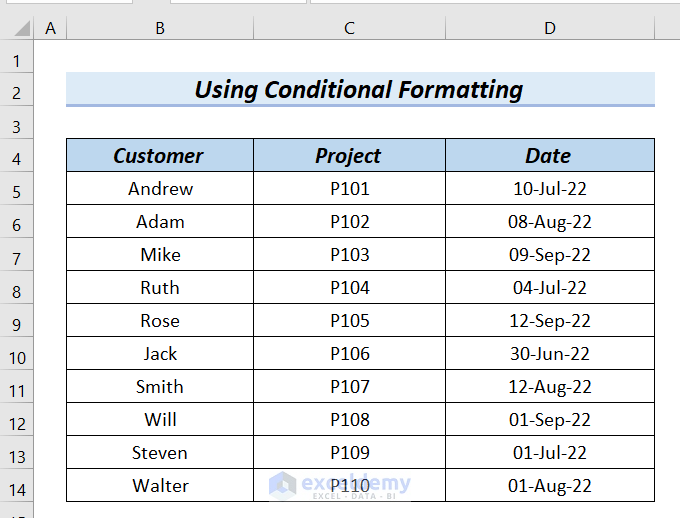
The following table has Customer, Project, and Date columns. We will use the Conditional Formatting feature to find out the date that is 30, 60, and 90 days after today.
Steps:
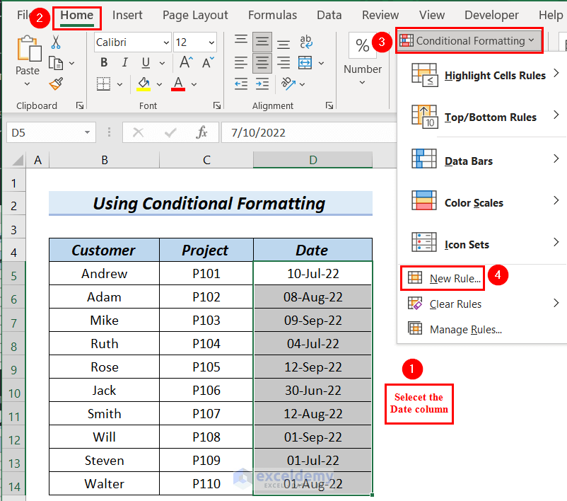
- Select the entire data in the Date column.
- Go to the Home tab, select Conditional Formatting, and select New Rule.
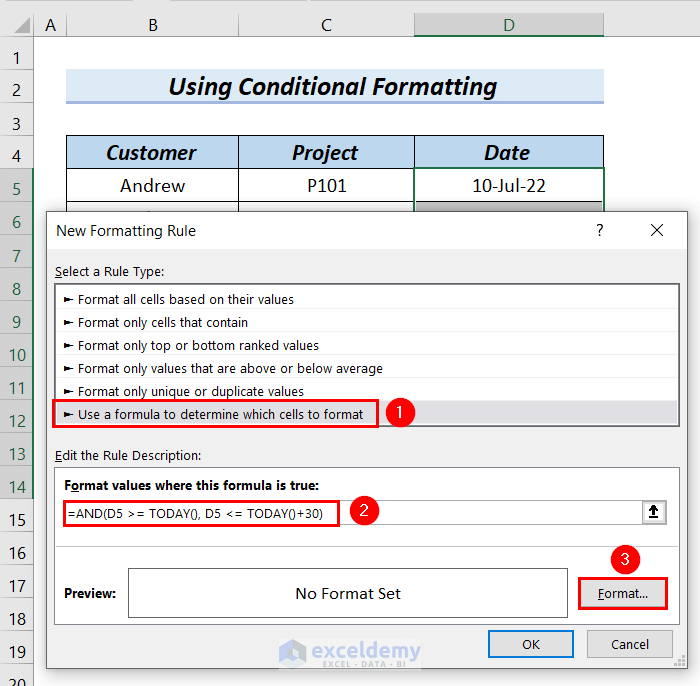
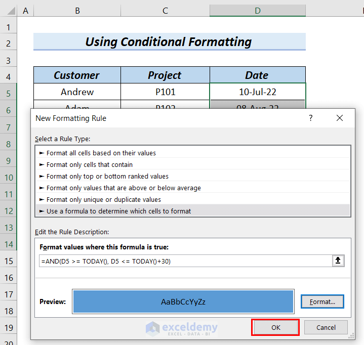
- A New Formatting Rule dialog box will appear.
- Select Use a formula to determine which cells to format.
- Use the following formula in the Format values where this formula is true box.
=AND(D5 >= TODAY(), D5 <= TODAY()+30)- Click on Format.
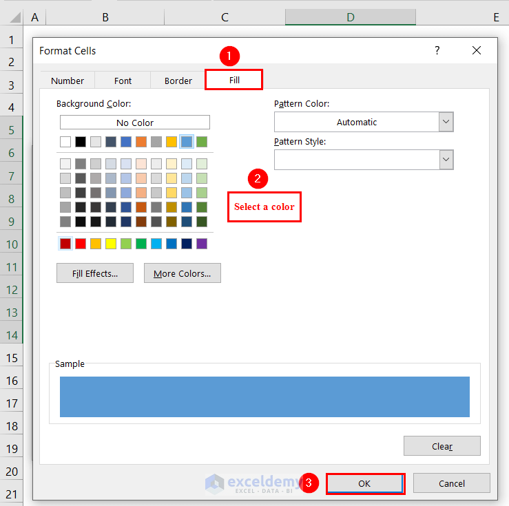
- A Format Cells dialog box will appear.
- Select Fill and select a color. We chose a blue color and you can see the preview below.
- Click OK.
- Click OK in the New Formatting Rule window.
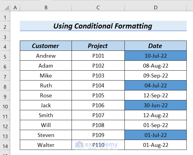
- We will see that all the dates that are at most 30 days away from today have been marked with blue color.
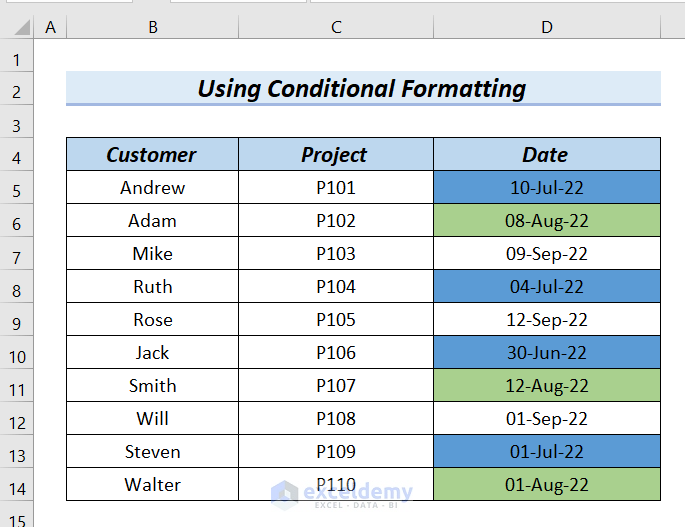
To highlight the dates that are 60 days away from today.
- Repeat the process above to go to conditional formatting.
- Use the following formula in the formula box for conditional formatting.
=AND(D5 >= TODAY()+30, D5 <= TODAY()+60)- Choose a different format color. We’ve chosen green.
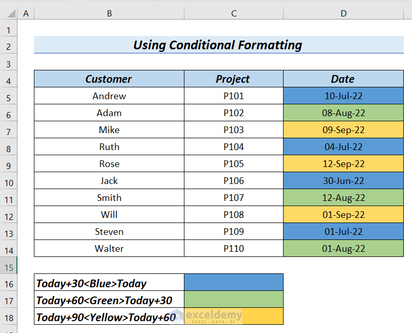
We will highlight the dates that are 90 days away from today.
- Use the following formula for formatting.
=AND(D5 >= TODAY()+60, D5 <= TODAY()+90)- Choose a third fill color (let’s say orange) for the format.
Method 2 – Adding 30, 60, and 90 Days in an Excel Aging Formula
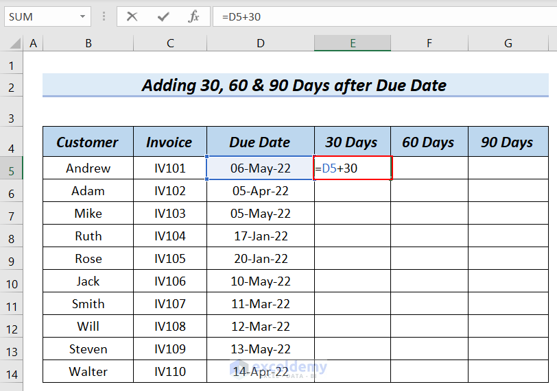
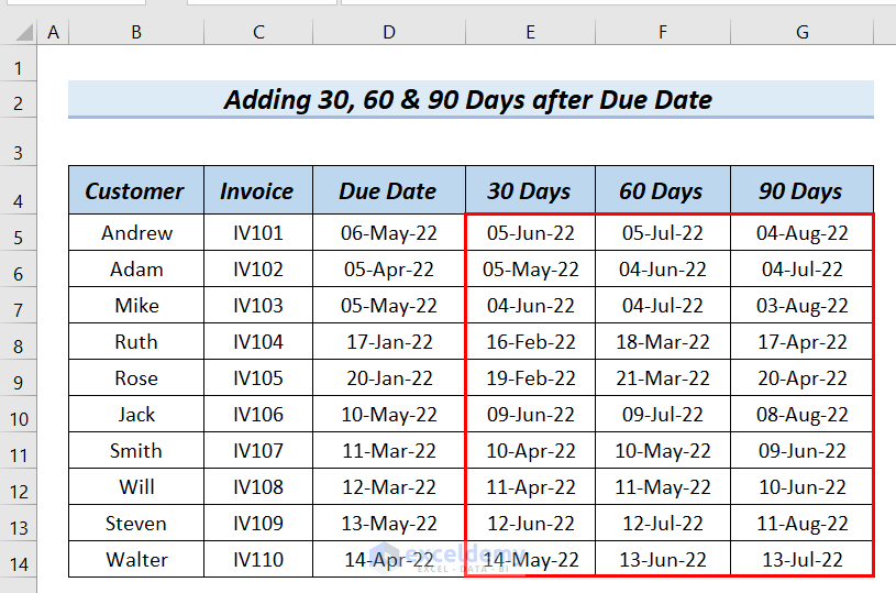
We will add 30 days, 60 days, and 90 days to the Due Date column with three result columns.
Steps:
- Use the following formula in cell E5.
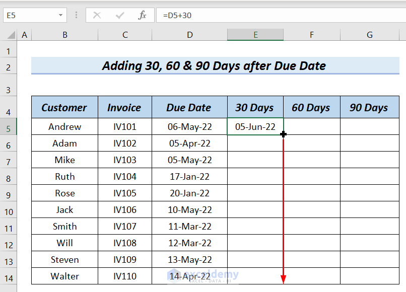
=D5+30This will simply add 30 days with the date of cell D5.
- Hit Enter and drag down the formula with the fill handle tool.
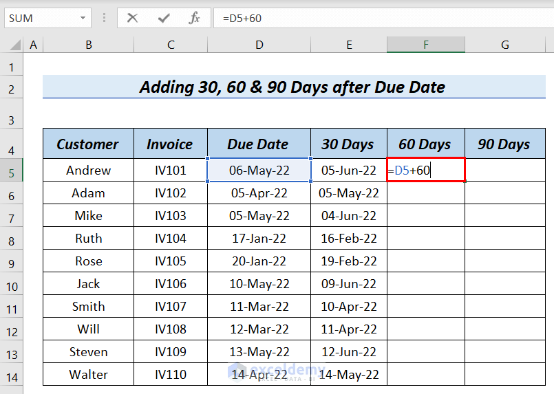
- Insert the following formula in cell F5.
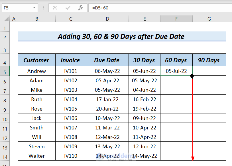
=D5+60This will simply add 60 days with the date of cell D5.
- Hit Enter and drag down the formula with the Fill Handle tool.
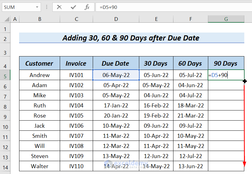
- Put the following formula in cell G5.
=D5+90This will add 90 days to the date of cell D5.
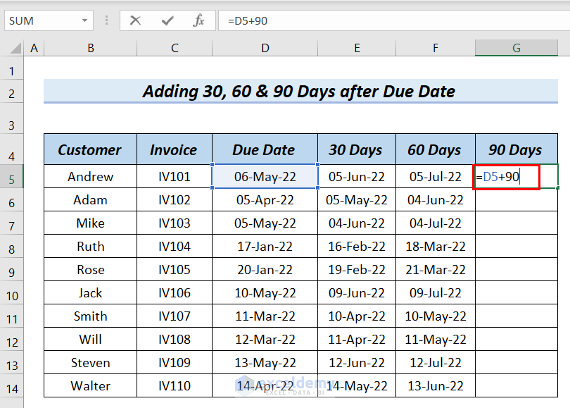
- Press Enter and drag down the formula with the Fill Handle tool.
- Here are the results.
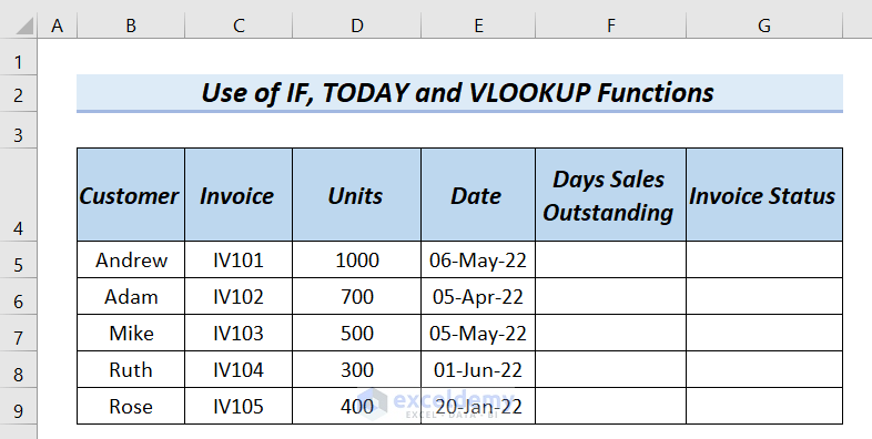
Method 3 – Use the IF, TODAY, and VLOOKUP Functions
The Date column contains the dates some invoices were due on. We will use calculate the Days Sales Outstanding and find out the Invoice Status.
Steps:
- Use the following formula in cell F5.
=IF(TODAY()>E5,TODAY()-E5,0)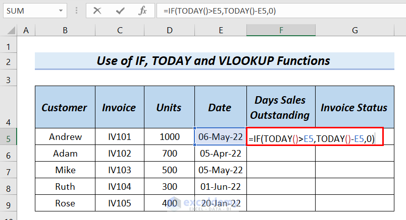
Formula Breakdown
- E5 is the invoice date.
- TODAY() function will return today’s date which is 14-06-22.
- IF function will return 0 if the difference between Today() and E5 is negative, otherwise the Days Sales Outstanding value will be equal to the difference between Today() and E5.
- Output: 39
- Press Enter.
- Drag down the formula with the Fill Handle tool.
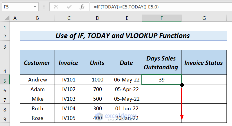
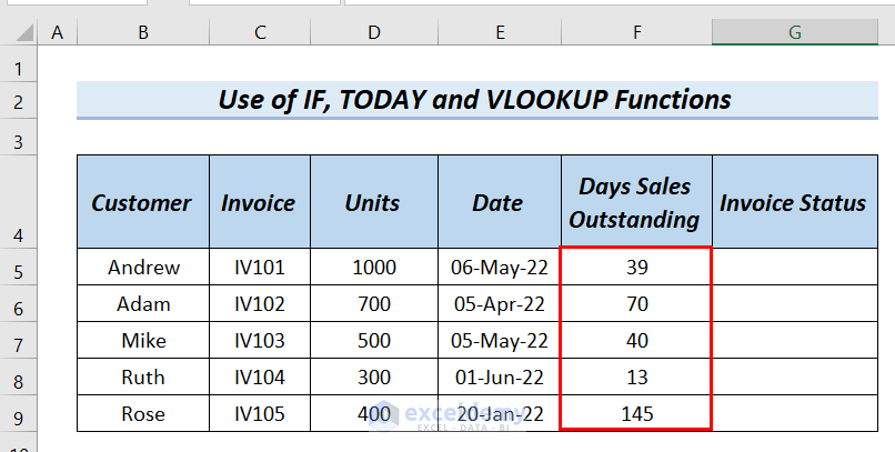
- We get the complete Days Sales Outstanding column.
- We have created the Days Category table. This has the categories of the invoice in the Category column according to their Days Sales Outstanding column to dictate the condition. We will use this Days Category table as table_array in the VLOOKUP function.
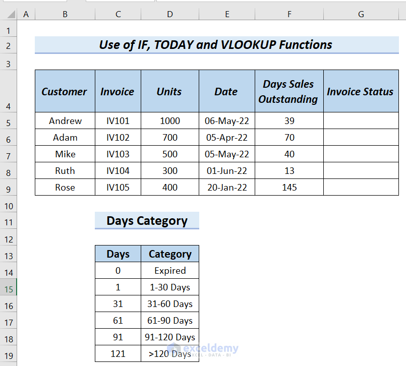
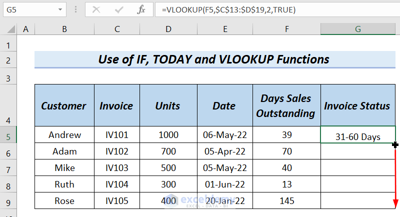
- Use the following formula in cell G5.
=VLOOKUP(F5,$J$4:$K$10,2,TRUE)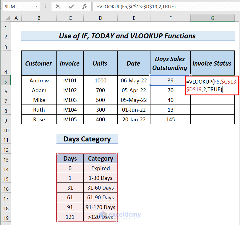
Formula Breakdown
F5 is the lookup_value that we are going to look up in the Category named range.
- $J$4:$K$10 is the table_array.
- 2 is the col_index_num.
- TRUE is for an approximate match.
- Output: 31-60 Days.
- Press Enter.
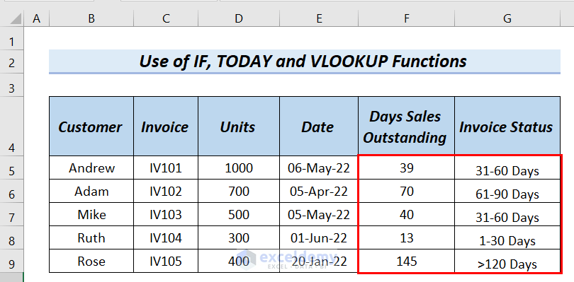
- Drag down the formula with the Fill Handle tool.
- Here are the results.
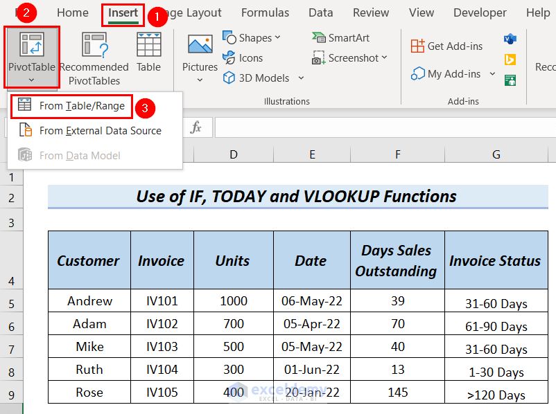
Let’s insert a pivot table to show the results.
- Go to the Insert tab.
- Select PivotTable and choose From Table/Range.
- A PivotTable from table or range dialog box will appear.
- Click on the arrow for Table/Range.
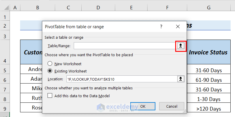
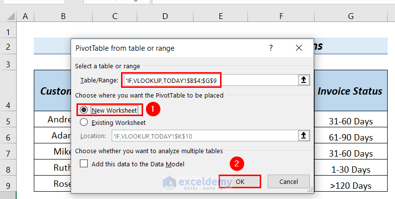
- Select your dataset and click the arrow again.
- Check New Worksheet.
- Click OK.
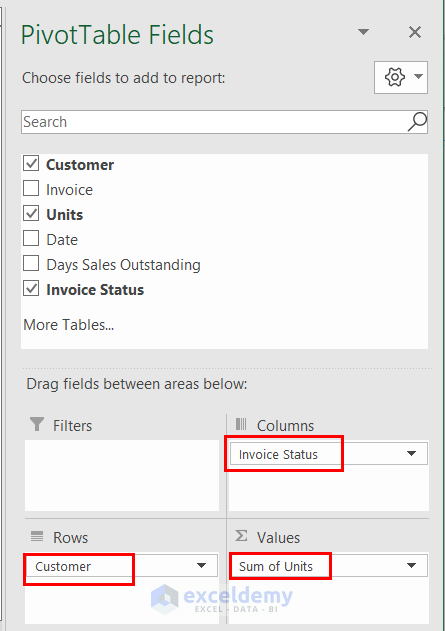
- A PivotTable Fields window appears.
- Drag Customer to the Rows area, Units to the Values area, and Invoice Status to the Columns area.
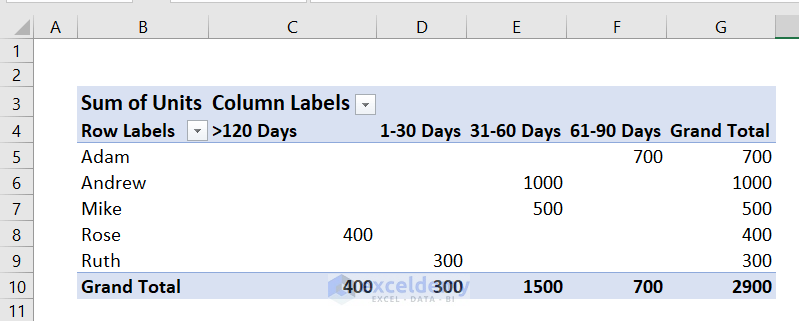
- We can see the pivot table.
Method 4 – Applying Addition and the TODAY Function to Find Upcoming Days
Steps:
- Enter the following formula in cell C6.
=TODAY()+30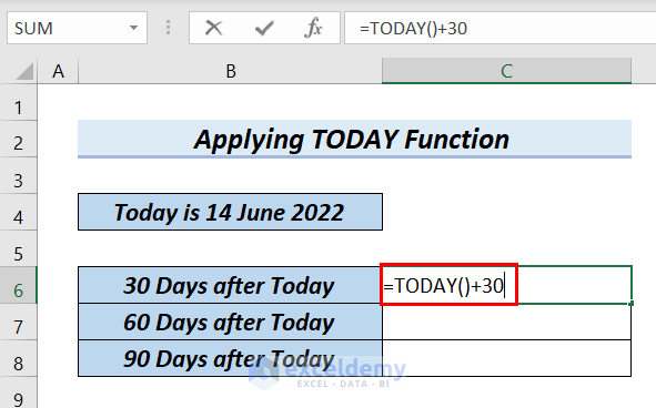
Formula Breakdown
- TODAY() → returns the date for today which is 14 June 2022.
- TODAY()+30 → adds 30 days with 14 June 2022.
- Output: 7/14/2022
- Insert the following formula in cell C7.
=TODAY()+60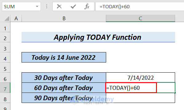
Formula Breakdown
- TODAY() → returns the date for today which is 14 June 2022.
- TODAY()+60 → adds 60 days with 14 June 2022.
- Output: 8/13/2022
- Enter the following formula in cell C8.
=TODAY()+90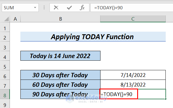
Formula Breakdown
- TODAY() → returns the date for today which is 14 June 2022.
- TODAY()+90 → adds 90 days with 14 June 2022.
- Output: 9/12/2022
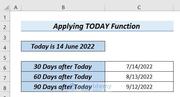
- Here are the results after applying the formulas.
Method 5 – Using Subtraction and the TODAY Function to Find the Previous Days
Steps:
- Use the following formula in cell C6.
=TODAY()-30- Hit Enter.
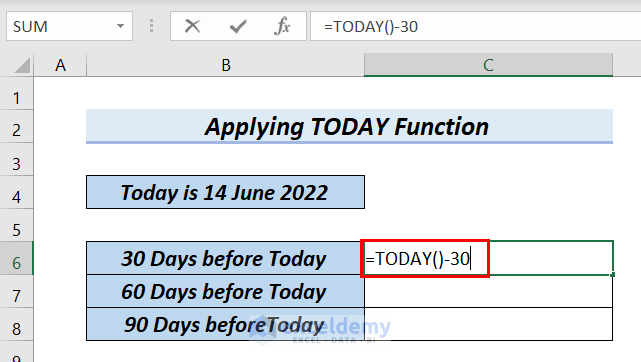
Formula Breakdown
- TODAY() → returns the date for today which is 14 June 2022.
- TODAY()-30 → subtracts 30 days from 14 June 2022.
- Output: 5/152022
- Use the following formula in cell C7.
=TODAY()-60- Hit Enter.
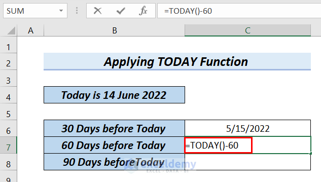
Formula Breakdown
- TODAY() → returns the date for today which is 14 June 2022.
- TODAY()-60 → subtracts 60 days from 14 June 2022.
- Output: 4/15/2022
- Insert the following formula in cell C8.
=TODAY()-90- Hit Enter.
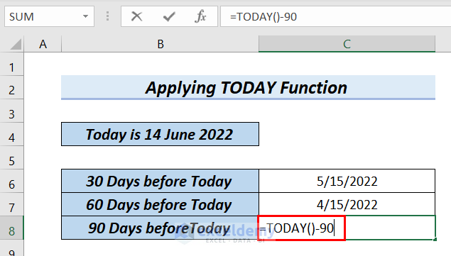
Formula Breakdown
- TODAY() → returns the date for today which is 14 June 2022.
- TODAY()-90 → subtracts 90 days from 14 June 2022.
- Output: 3/16/2022
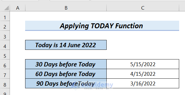
- Here are the results.
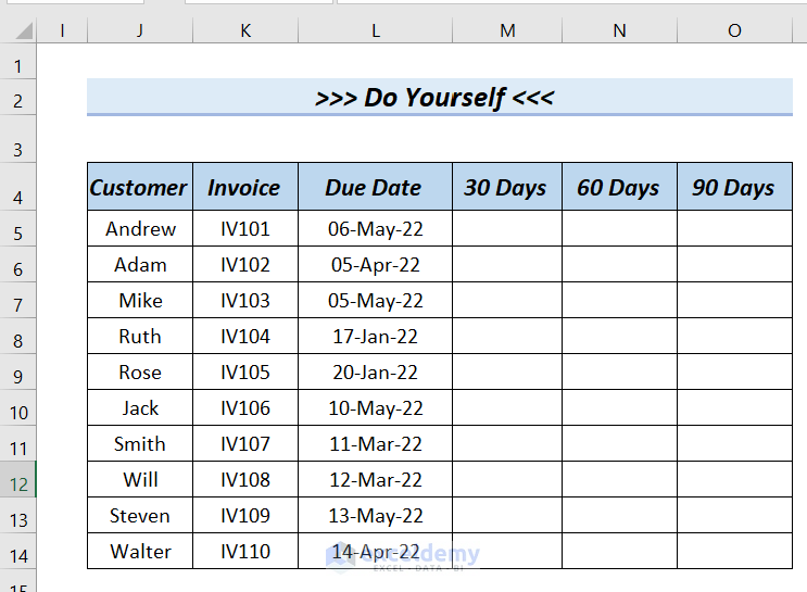
Practice Section
We’ve included a practice sheet you can use to test these methods.
Download the Practice Workbook
<< Go Back to Ageing | Formula List | Learn Excel
Get FREE Advanced Excel Exercises with Solutions!

Thank you for your valuable tutorials on your website, but it would be great if your content could be used for free.
Afia Aziz, since you are a Muslim, give as charity to the lessons so that you can get what you want from Allah.
Hello Mohammed.
Thanks for your appreciation. Our content is completely free for our users learning but don’t use it for your business purpose without proper agreement.
Regards
ExcelDemy
Hi ,
Please send me the excel template with the formula .
[email protected]
Hello Abdul,
Excel file is given in the download section of the article. You also can download the template with formula from this link : Ageing Formula 30 60 90 Days.xlsx
Regards
ExcelDemy