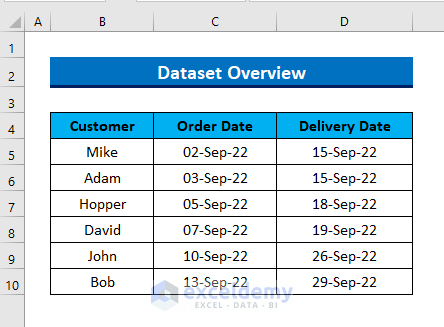
Case 1 – Calculate Days Between Specific Dates
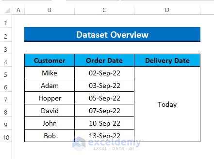
Let’s say we have a sample dataset of names of some customers who have ordered some products from a shop, the order date, and the delivery date. We want to calculate the days taken to deliver the products to the customers.
Method 1 – Subtracting Days
Steps:
- Create a new column for the results.
- Select the first cell in that column and apply the following formula:
=D5-C5
- Press Enter.
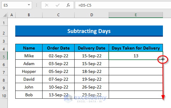
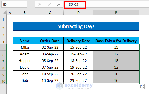
- Drag the Fill Handle tool to Autofill the formula down to the next cells and all the cells will calculate the days taken for delivery and return the results.
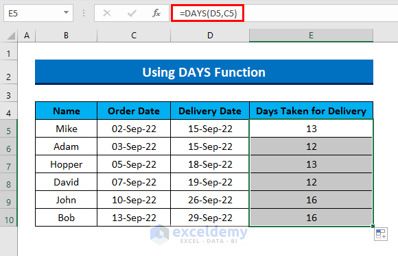
Method 2 – Calculate Using DAYS Function
The DAYS function returns the number of days between two specific days.
Steps:
- Select a cell and type the following formula into the selected cell:
=DAYS(D5,C5)
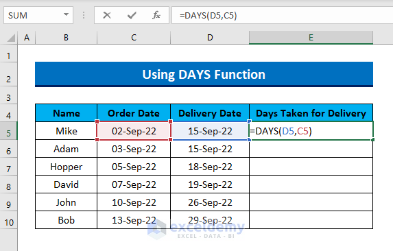
- Press Enter and drag the formula to the next cells to copy the formula and calculate the days.
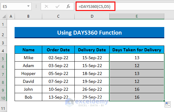
Method 3 – Using DAYS360 Function
The DAYS360 function can better approximate fiscal months.
Steps:
- Select E5 and type the following formula:
=DAYS360(C5,D5)
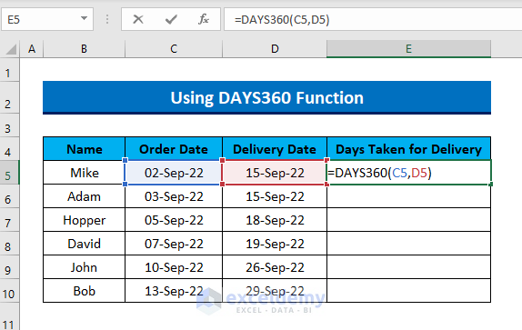
- Press Enter and drag the formula down to get the output for all cells.
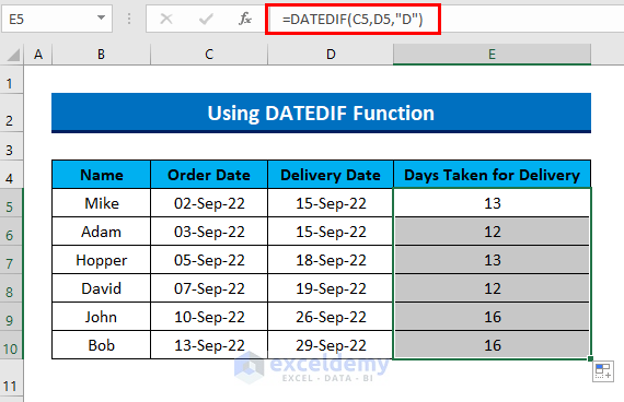
Method 4 – Applying DATEDIF Function
Steps:
- Type the following formula in E5:
=DATEDIF(C5,D5,"D")
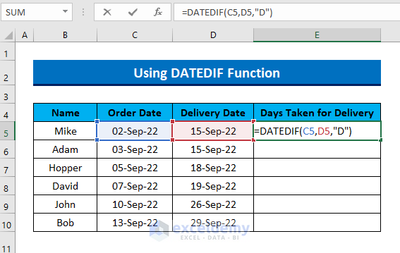
- Press Enter and the cell will return the result.
- Drag the formula down and all the cells will calculate the days between the two dates and return you the output.
Method 5 – With YEARFRAC Function
Steps:
- Select E5 and copy the following formula:
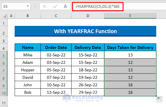
=YEARFRAC(C5,D5,3)*365
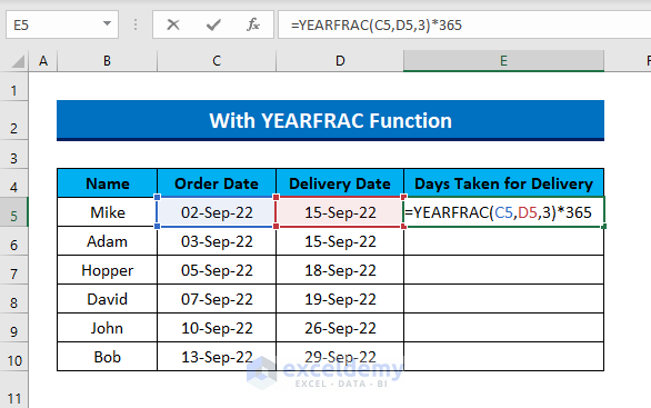
- Press Enter to let the cell show the result.
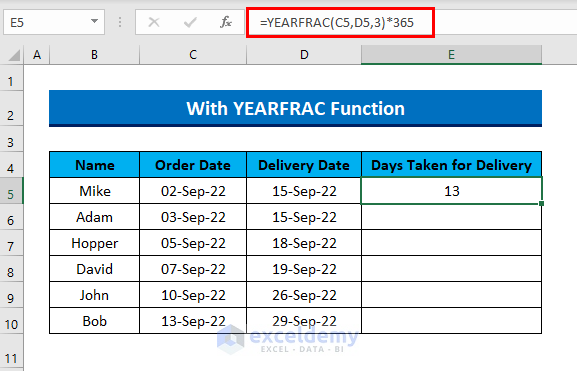
💡 Formula Breakdown
YEARFRAC(C5,D5,3) returns the actual year considering 365 days as the basis is used 3 (365 day count basis).
Output=> 0.0356164383561644
YEARFRAC(C5,D5,3)*365 = 0.0356164383561644*365 will convert the year into days.
So, final Output=> 13
- Drag the formula down and all the cells will return the result.
Case 2 – Aging Formula to Calculate Days from Current Date
Another case for calculating days is when one date is specified and another date is the current date. The scenario from the sample would be like the following screenshot, so we’ll remove the D column and use it for the results.
Method 1 – Applying TODAY Function
Steps:
- Select D5 and type the following formula into the cell.
=TODAY()-C5
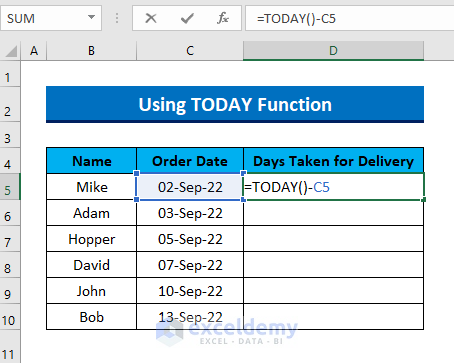
- Since TODAY function returns the current date, subtracting the specified date from this function results in the difference between them.
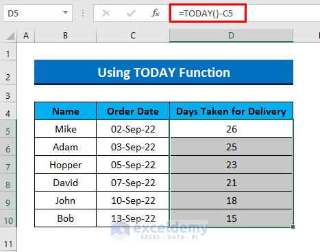
Screenshot was taken on Sept 28, 2022, which was the result of the TODAY() function.
Method 2 – Combining YEARFRAC and TODAY Functions
- Use the following formula in D5:
=YEARFRAC(C5,TODAY(),3)*365
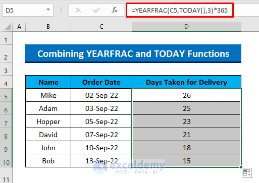
Screenshot was taken on Sept 28, 2022, which was the result of the TODAY() function.
💡 Formula Breakdown
TODAY() function returns the date of today. Sept 28, 2022 for the time of writing.
YEARFRAC(C5,TODAY(),3) returns the actual year considering 365 days as the basis is used 3 (365-day count basis).
YEARFRAC(C5,TODAY(),3)*365 will convert the year into days.
So, final Output=> 26
Things to Remember
- Change the format of the cell after applying the formula if the cell shows the result in date format.
Download Practice Workbook
You can download the practice book from the link below.
<< Go Back to Ageing | Formula List | Learn Excel
Get FREE Advanced Excel Exercises with Solutions!
