Step 1 – Create the Dataset
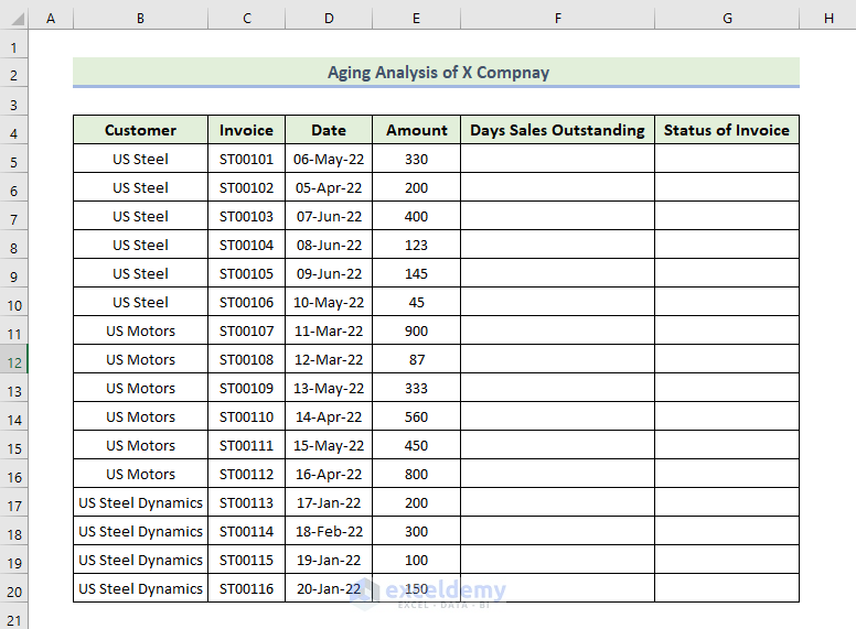
- In the following image, you can see the basic dataset of the Aging Analysis report.
- We have Customer names, Invoice numbers, Date, and Amount.
- We have inserted the columns Days Sales Outstanding and Status of Invoice.
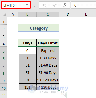
- Create the categories of the invoice according to their day’s sales outstanding to dictate the condition.
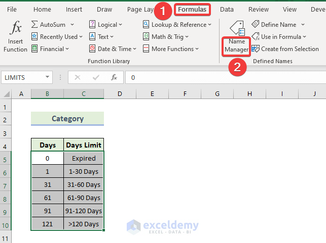
- Select the cells and go to the Formulas tab, then select Name Manager.
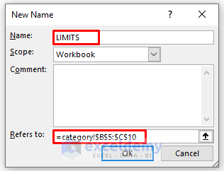
- When the New Name dialog box appears, enter the name as LIMITS in the Name box.
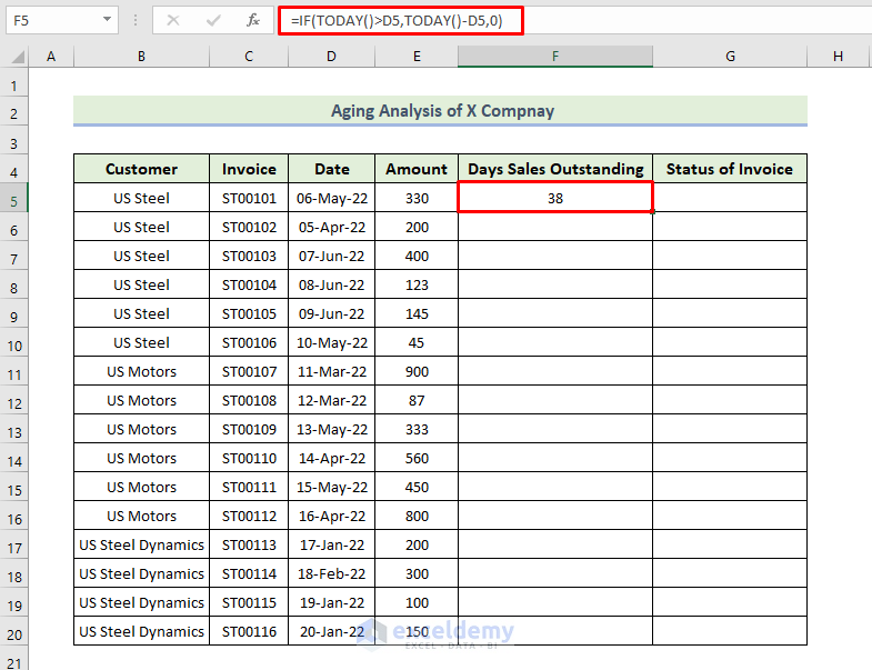
Step 2 – Use Formulas for the Aging Analysis
- To calculate days sales outstanding, use the following formula in cell F5:
=IF(TODAY()>D5,TODAY()-D5,0)
- Press Enter.
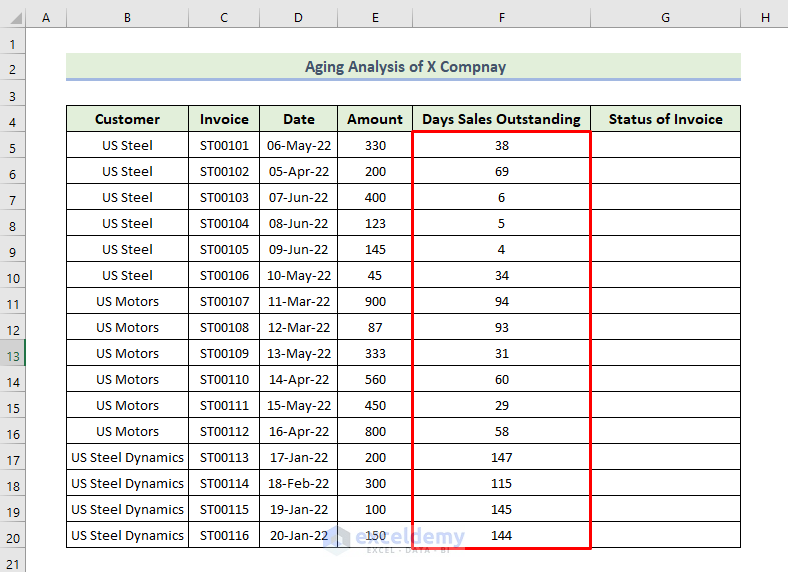
- Dag the Fill handle icon down to fill the column.
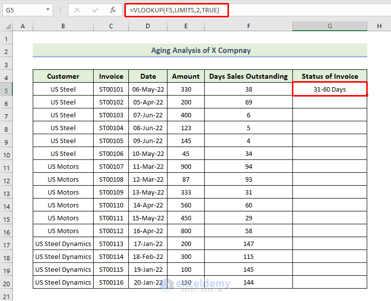
- To determine the status of the invoice, use the following formula in the cell F5:
=VLOOKUP(F5,LIMITS,2,TRUE)
- Press Enter.
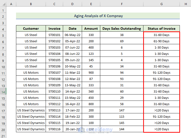
- Drag the Fill handle icon down.
Step 3 – Create a Pivot Table for an Aging Analysis Summary
- Select the dataset.
- Go to the Insert tab and select PivotTable.
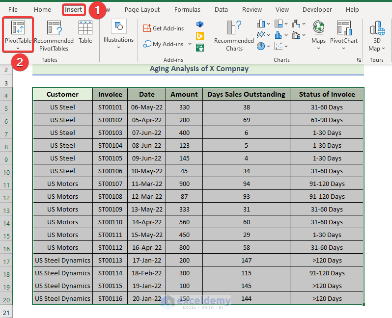
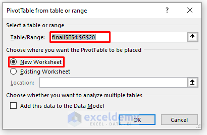
- In the PivotTable from table or range dialog box, choose New Worksheet.
- Click on OK.
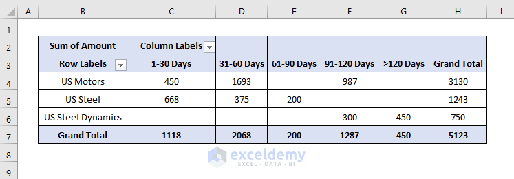
- In the PivotTable Fields window, drag Customer to the Rows area, Amount to the Values area, and Status of Invoice to the Columns area.
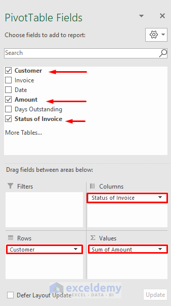
- You will get the following pivot table.
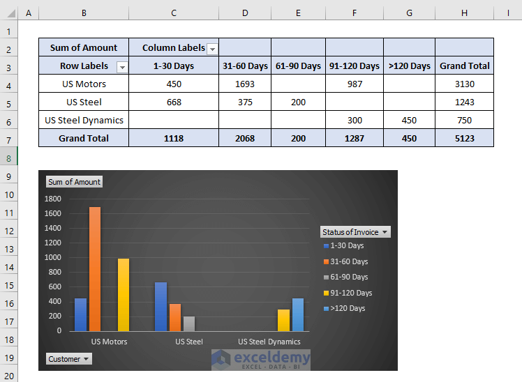
Step 4 – Generate a Dynamic Aging Analysis Report
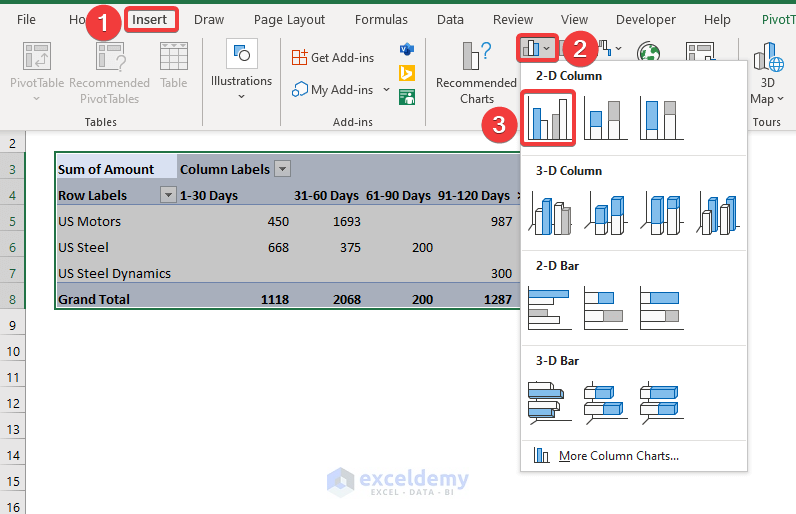
- Select the dataset and go to the Insert tab.
- Select the Clustered Column chart.
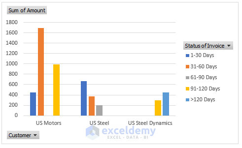
- You will get the following Clustered Column chart.
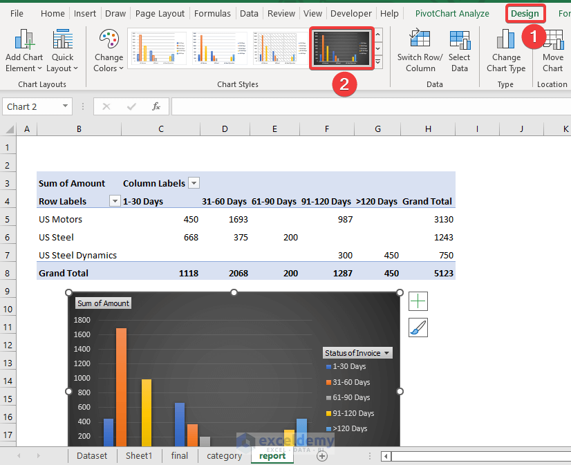
- Select Chart Design and select the Style 8 option from the Chart Styles group.
- You will get the following Clustered Column chart
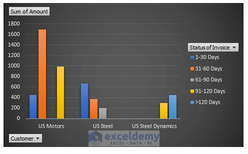
- Here’s the final result.
Things to Remember
✎ You have to adjust the row height after following each method.
Download the Practice Workbook
<< Go Back to Ageing | Formula List | Learn Excel
Get FREE Advanced Excel Exercises with Solutions!

Thank you. A first-timer doing the aging analysis and the tutorial is very helpful.
Glad to know it helped you!
Excellent, thanks a lot
Hello Sirajudeen,
You are most welcome.
Regards
ExcelDemy
Excellent Workbook, Thank you for the assistance. I am going to start using it to keep track of my outstanding payment to suppliers and customers receipts.
Hello Moegamat Shakier Stuurman,
You are most welcome. Thanks for your appreciation. Glad to hear that you are going to use it to track aging analysis. Keep exploring Excel with ExcelDemy!
Regards
ExcelDemy
when I make pivot table as per your guidance, >120 comes in the first column whereas it should be in the last. What to do?
Hello Muhammad Q Naeem,
By default, Pivot Tables sort column labels alphabetically, which places “>120” first. To fix this and show the aging buckets in logical order (e.g., “0-30”, “31-60”, …, “>120”), follow these steps:
1. Right-click any column label in the Pivot Table.
2. Click Sort > More Sort Options.
3. Choose Manual and then drag the “>120” column to the end.
Alternatively, create a custom list for aging categories (e.g., “0-30”, “31-60”, “61-90”, “91-120”, “>120”) and use it in your Pivot Table sort settings:
1. Go to File > Options > Advanced > General > Edit Custom Lists.
2. Add your desired order, then sort by that list.
This will ensure the aging columns appear in the proper sequence.
Regards
ExcelDemy
Thank you very much. I got it.
But there is an other question. When I apply formula using SUMIFS (with some other condition) it does not provide sum where >121 used. For other below >121 condition, it is ok.
Hello Muhammad Q Naeem,
You are most welcome. Solved your issue, hopefully it will work.
Regards
ExcelDemy
When I use SUMIFS, it does not work on >121. What to do in this case.
Aging RAS
Govt PIF Pvt Corp
0-30 463,743.25 193,093.86 868,907.80
31-60 – – 299,850.00
61-90 235,996.27 100,337.50 151,800.00
91-120 184,575.00 60,375.00 146,894.71
>121 – – –
TOTAL 884,314.52 353,806.36 1,467,452.51
Hello Muhammad Q Naeem,
When using SUMIFS to sum values greater than 121 (e.g., for an aging bucket “>121”), make sure your formula uses the correct criteria syntax. For example, if your “Aging” column is Column A and your values are in Column B, your formula should look like:
=SUMIFS(B:B, A:A, “>121”)
Common issues: Check that the values in your “Aging” column are actual numbers, not text. If they are text (e.g., “>121” as a label), SUMIFS won’t match them as numbers.
For aging analysis, create a helper column that actually calculates the numeric age (e.g., days overdue). Then, use SUMIFS on that column.
Example: If you have a calculated column for “Days Overdue,” your formula for the “>121” bucket should be:
=SUMIFS(B:B, C:C, “>121”)
(where C:C is your numeric “Days Overdue” column.)
If your bucket is a text like “>121”, use SUMIF with the bucket label:
=SUMIF(A:A, “>121”, B:B)
But the best approach is to calculate days overdue as numbers, then use SUMIFS with numeric criteria.
Regards
ExcelDemy