Dataset Overview
In Microsoft Excel, we often need to determine the age or duration of various items. Additionally, there are cases where we want to exclude weekends from the calculation. If you’re puzzled about how to achieve this with specific criteria, this article will guide you through four suitable methods for calculating the days between certain dates while excluding weekends.
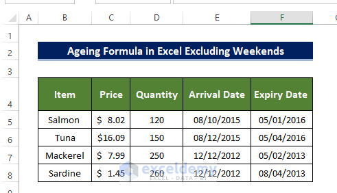
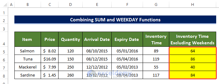
For the demonstration purpose we are going to use the below dataset, In the dataset, we got the fish items listed in the Item column and the Price, Quantity, Arrival Date, and Expiry Date in their respective columns. We are going to calculate the workdays in between the dates excluding the weekends.
Method 1 – Combination SUM and WEEKDAYS Functions
Objective: Calculate the inventory time for fish items listed in the dataset, considering their Arrival Date and Expiry Date columns.
Steps
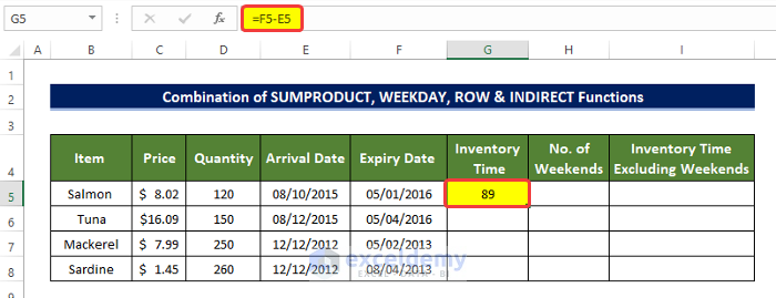
- Select cell G5 and enter the formula for the interval:
=F5-E5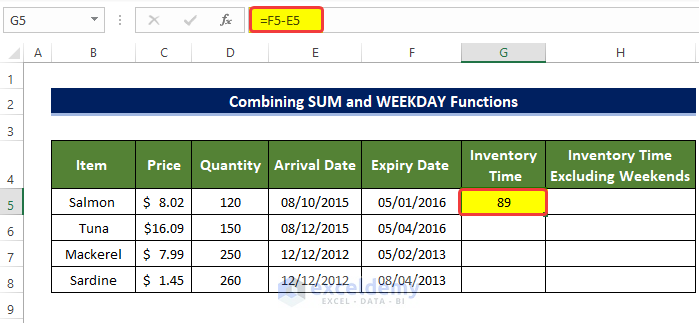
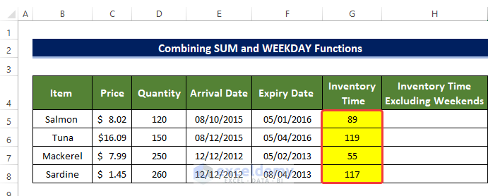
- Drag the Fill Handle down to fill cells G6:G8 with the formula.
- Select cell H5 and enter the following formula to calculate the inventory time (excluding weekends):
=SUM(INT((WEEKDAY(E5-{2,3,4,5,6})+F5-E5)/7))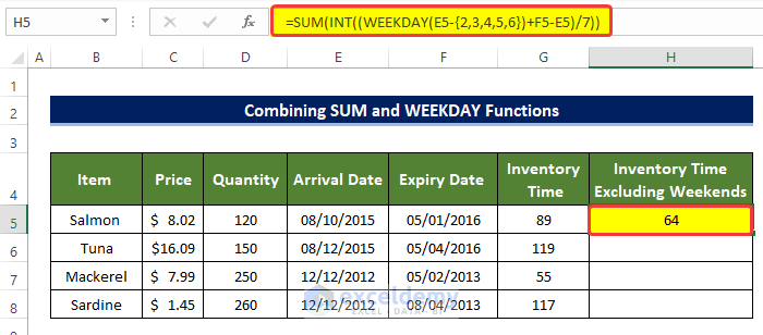
- Drag the Fill Handle down to fill cells H6:H8 with the inventory time for each fish item.
How Does the Formula Work?
- WEEKDAY(E5-{2,3,4,5,6}): This function returns the weekday number for the Arrival Date, adjusted for Monday to Friday (excluding weekends).
- (WEEKDAY(E5-{2,3,4,5,6}) + F5 – E5): Adds the total interval days to the weekday values obtained in the previous step.
- INT((WEEKDAY(E5-{2,3,4,5,6}) + F5 – E5) / 7): Divides the result by 7 to find the number of weeks each weekday contributes. Some values may be decimals, but the INT function converts them to integers.
- SUM(INT((WEEKDAY(E5-{2,3,4,5,6}) + F5 – E5) / 7)): Finally, this formula sums up the array of values obtained in the previous step.
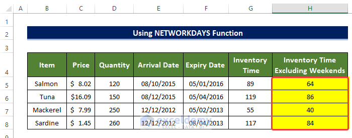
Method 2 – Using the NETWORKDAYS Function
In this method, we’ll utilize the NETWORKDAYS function to extract workdays between inventory dates.
Steps
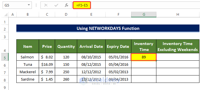
- Select cell G5 and enter the following formula:
=F5-E5This calculates the number of days between the Arrival and Expiry dates, including weekends.
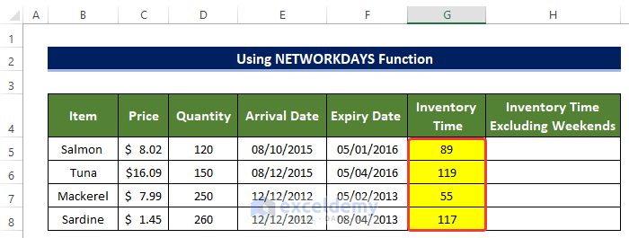
- Drag the Fill Handle down to fill cells G6:G8 with the interval values.
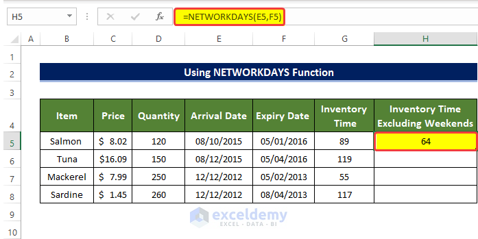
- Select cell H5 and enter the following formula:
=NETWORKDAYS(E5,F5)This provides the inventory time for fish items in the Item column (cell B5), excluding weekends.
- Drag the Fill Handle down to fill cells H6:H8 with the inventory time for each fish item.
Note:
The NETWORKDAYS function considers weekends as Saturday and Sunday. If your weekends differ in your region, consider using the NETWORKDAYS.INTL function.
Method 3 – Utilizing NETWORKDAYS.INTL Function
The NETWORKDAYS.INTL function extends the NETWORKDAYS functionality to account for specific weekend days.
Steps
- Select cell G5 and enter the following formula:
=F5-E5Calculate the days between Arrival and Expiry Dates, including weekends.
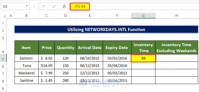
- Drag the Fill Handle down to fill cells G6:G8 with the interval values.

- Select cell H5 and enter the following formula:
=NETWORKDAYS.INTL(E5,F5,1)This provides the inventory time for fish in the Item column (cell B5), excluding weekends.
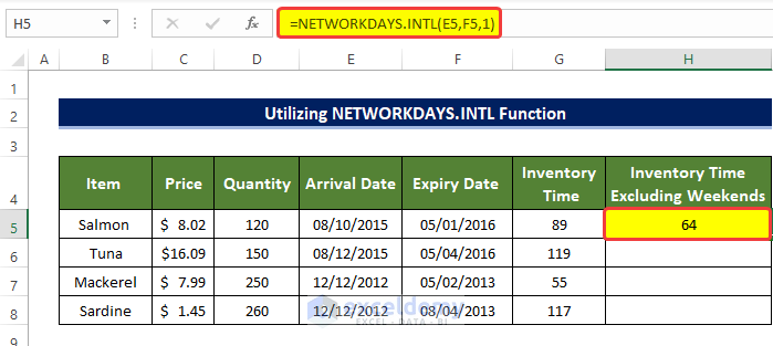
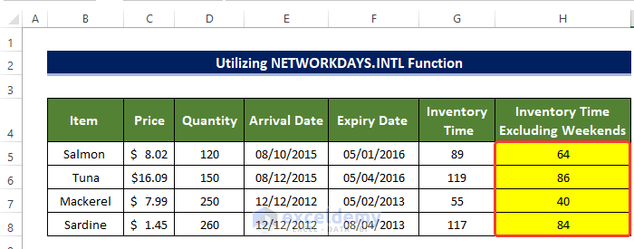
- Drag the Fill Handle down to fill cells H6:H8 with the inventory time.
Note
The last argument in the formula specifies which days are considered weekends. The default is Saturday and Sunday. Adjust this based on your region.
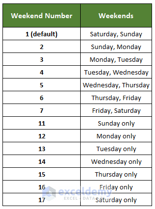
If you do not mention any number, then the default is set to Saturday and Sunday. You need to choose your desired one from the list above.
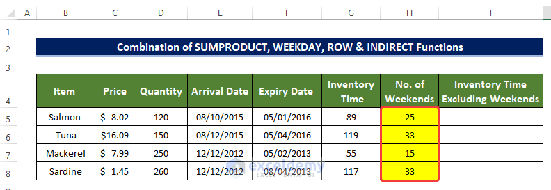
Method 4 – Combining SUMPRODUCT, WEEKDAY, ROW, and INDIRECT Functions
This method counts workdays (excluding weekends) between inventory times using a combination of functions.
Steps
- Select cell G5 and enter the following formula:
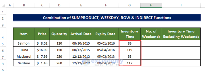
=F5-E5Calculate the days between Arrival and Expiry Dates, including weekends.
- Drag the Fill Handle down to fill cells G6:G8 with the interval values.
- Select cell H5 and enter the following formula:
=SUMPRODUCT(--(WEEKDAY(ROW(INDIRECT(E5&":"&F5)),2)>5))-1This counts the number of weekends between the inventory times.
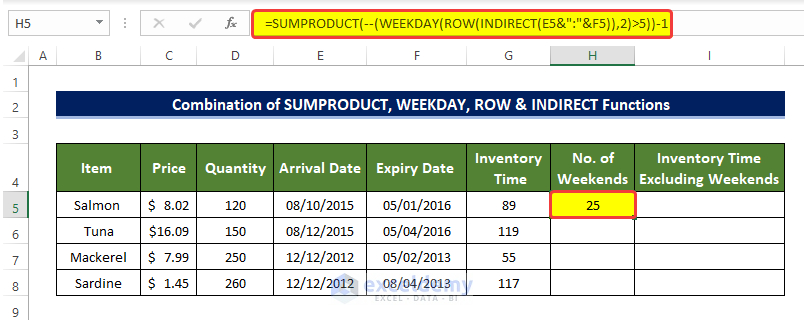
- Drag the Fill Handle down to fill cells H6:H8 with the weekend count.
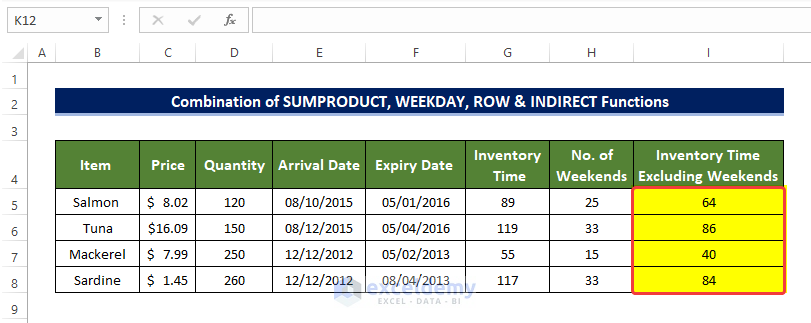
- Select cell I5 and enter:
=G5-H5This calculates the inventory time for fish items, excluding weekends.
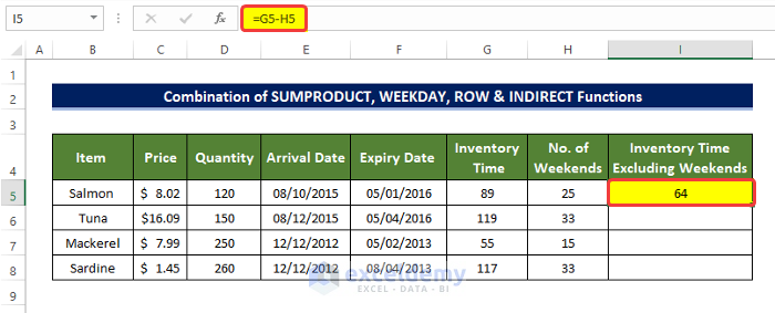
- Drag the Fill Handle down to fill cells I6:I8 with the inventory time.
How Does the Formula Work?
- INDIRECT(E5&“:”&F5):
- The INDIRECT function converts the Arrival date and Expiry date into a range.
- It creates a reference to all the dates between cell E5 and F5.
- ROW(INDIRECT(E5&“:”&F5)):
- This formula returns the row numbers corresponding to the dates in the specified range.
- Essentially, it lists all the dates vertically.
- WEEKDAY(ROW(INDIRECT(E5&“:”&F5)), 2):
- The WEEKDAY function returns the numerical representation of each day of the week.
- Here, 1 represents Monday, 2 represents Tuesday, and so on, up to 7 (Sunday).
- (WEEKDAY(ROW(INDIRECT(E5&“:”&F5)), 2) > 5):
- This part of the formula evaluates whether the weekday value is greater than 5 (i.e., Saturday or Sunday).
- If the value is greater than 5, it returns True; otherwise, it returns False.
- By doing this, we filter out weekends (True values).
- SUMPRODUCT(–(WEEKDAY(ROW(INDIRECT(E5&“:”&F5)), 2) > 5)) – 1:
- The SUMPRODUCT function counts the number of True values obtained from the previous step.
- The double dash (– –) converts True to 1 and False to 0.
- Subtracting 1 accounts for the extra weekend counted.
Download Practice Workbook
You can download the practice workbook from here:
<< Go Back to Ageing | Formula List | Learn Excel
Get FREE Advanced Excel Exercises with Solutions!
