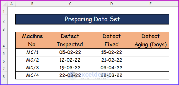
Method 1 – Preparing Data Set
- Make an extra column along the main data set under column E.
- Name the column Defect Aging.
- Apply the formula to calculate the result in days.
Method 2 – Applying Formula to Calculate Defect Aging
- Use the following combination formula of the IF function and the TODAY function in cell E5.
=IF(D5<>"",D5-C5,TODAY()-C5)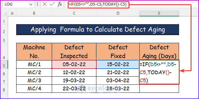
Formula Breakdown
=IF(D5<>””,D5-C5,TODAY()-C5)
- The IF function will see if cell D5 is empty or not.
- If it finds the cell value, it will subtract it from the cell value of D5 to calculate the date.
- If it finds no value in C5, it will delete the current date from D5.
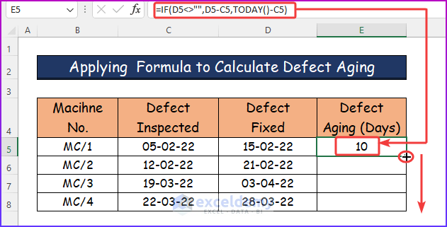
- Press Enter to get the desired result in cell E5, showing defect aging for the first machine, which is 10 days.
- Use the AutoFill feature to drag the same formula for the lower cells of that column.
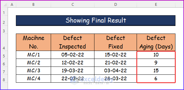
Method 3 – Showing Final Result
- Applying AutoFill, the formula will get adjusted for the lower cells from cell E6:E8.
- You can see the values of defect aging for all the machines.
Applying Aging Formula in Excel Using IF Function
Step 1:
- Take the following data set, which contains the names and ages of some random people in columns B and C, respectively.
- To know the age groups, insert the following nested IF formula in cell D5.
=IF(C5<16,"Children",IF(C5<=25,"Young Adults",IF(C5<35,"Middle-aged Adults","Senior Citizen")))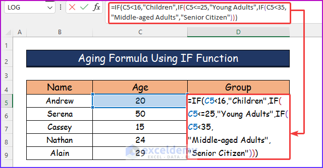
Formula Breakdown
=IF(C5<16,”Children”,IF(C5<=25,”Young Adults”,IF(C5<35,”Middle-aged Adults”,”Senior Citizen”)))
- IF(C5<16,“Children” …): This formula denotes if the value of cell C5 is less than 16, which means if the age is less than 16, then it will return a string “Children”. It shows that people with the age below 16 will be in the Children group.
- IF(C5<=25,“Young Adults” ….): This part means if the value of cell C5 doesn’t meet the first condition, it will automatically consider this second condition. The second condition demonstrates if the value of cell C5 is less than or equal to 25, it will return a string called “Young Adults”. This actually denotes age limit of less than or equal to 25 will be in the Young Adults group.
- IF(C5<35,“Middle-aged Adults” ….): If the value of cell C5 doesn’t match the above two criteria then, it will go through this condition. This formula says if the value of C5 is less than 35, it will return a string called “Middle-aged Adults”. This demonstrates the age limit of less than 35 will be in the Middle-aged group.
- Finally, if the value of C5 doesn’t match any of the above criteria, it will automatically return a string “Senior Citizen”.So, if the age limit of C5 is above 35, it will be in the Senior Citizen group.
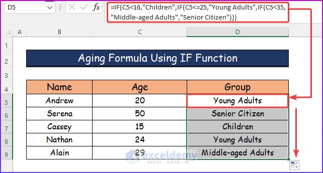
Step 2:
- Press Enter and see the age group for Andrew in cell D5 which is Young Adults.
- Drag the same formula to the lower cells of that column by using Fill Handle.
Applying Aging Formula in Excel for Days and Months
In the last section of this article, I will demonstrate the procedure to apply the aging formula to calculate days and months in Excel. It will also use a combination of some Excel functions that include the INT, YEARFRAC, and TODAY functions. The steps to apply this formula are as follows.
Step 1:
- To determine one’s age in days and months, I will use the following sample data set.
- We have the names and dates of birth of some random people.
- To calculate the age of the first person in days, type the following combination formula.
=INT((YEARFRAC(C5,TODAY(),1)*365))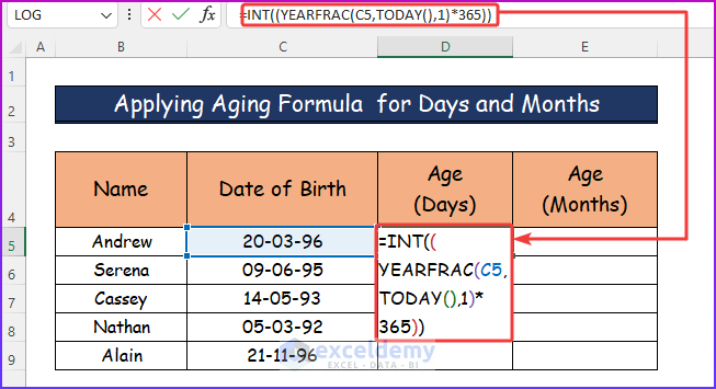
Formula Breakdown
=INT((YEARFRAC(C5,TODAY(),1)*365))
- YEARFRAC(C5,TODAY(),1): The YEARFRAC function will count the difference in the year between cell C5 and the current year in fractions.
- (YEARFRAC(C5,TODAY(),1)*365): Then, I will multiply the year by 365 to convert it into days.
- INT((YEARFRAC(C5,TODAY(),1)*365)): Lastly, the INT function will turn the fraction value into its nearest integer.
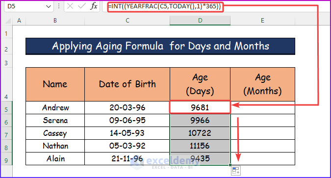
Step 2:
- Hit Enter to see the desired age in days.
- With the help of AutoFill use the same formula in the following column cells.
Step 3:
- To apply the aging formula for months, in cell E5, use the following combination formula.
- The applied formula is the same as the previous one, but in place of 365, will multiply the year value by 12 to convert it into months.
=INT((YEARFRAC(C5,TODAY(),1)*12))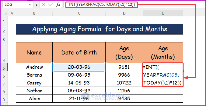
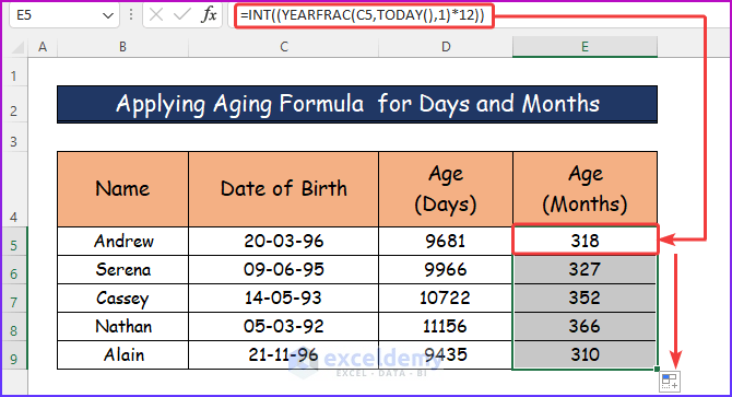
Step 4:
- After pressing Enter and dragging the Fill Handle, you will get the desired ages in months for everyone.
Download Practice Workbook
You can download the free Excel workbook here and practice on your own.
<< Go Back to Ageing | Formula List | Learn Excel
Get FREE Advanced Excel Exercises with Solutions!
