The Excel INT Function:
Summary
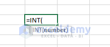
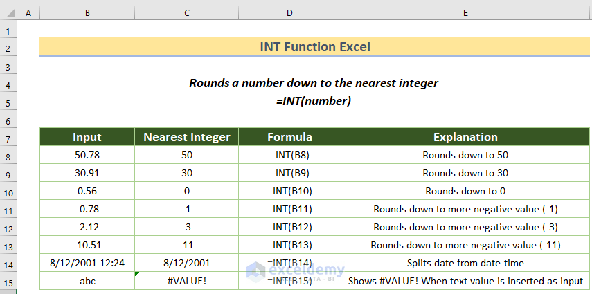
A decimal number can be represented as an integer using the INT function, which rounds it down to the lowest integer portion.
Syntax
Return Value
The rounded integer portion of a decimal number.
Arguments
| Argument | Required or Optional | Value |
|---|---|---|
| number | required | The real number from which you want to get an integer |
INT Function in Excel (Quick View)
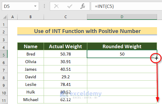
Example 1 – Using the INT Function for Positive Numbers
- Select a blank cell and enter the formula after an equal sign (=).
=INT(C5)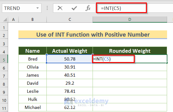
- Press ENTER.
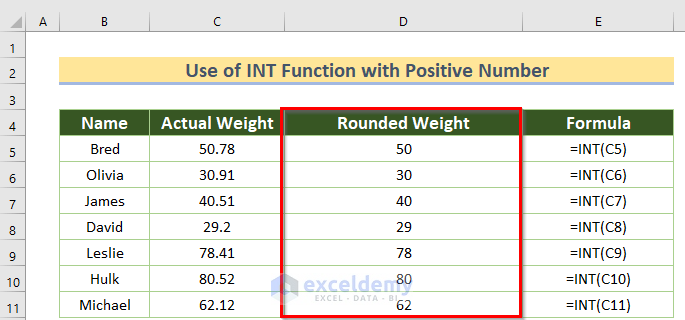
You will get the positive integer number rounded toward zero.
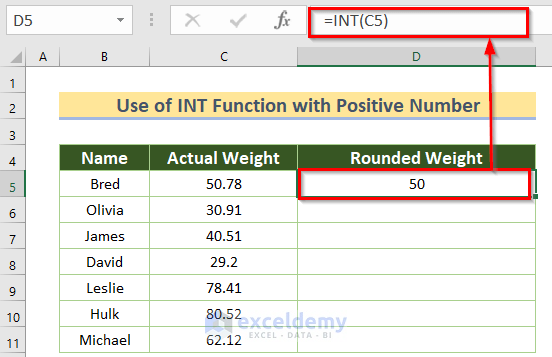
This is the output.
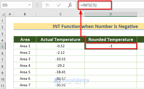
Example 2 – Use the INT Function for Negative Numbers
- Select D5 and enter the following formula.
=INT(C5)- Press ENTER.
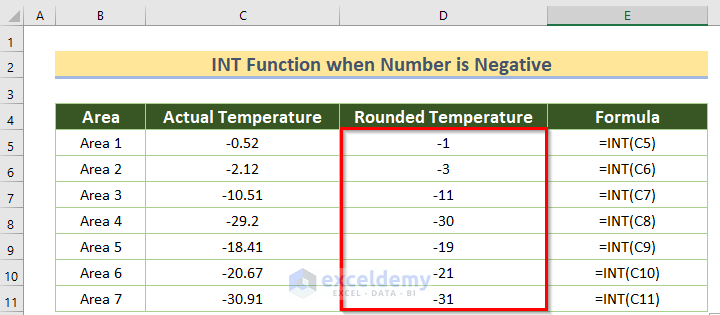
- Drag down the Fill Handle to see the result in the rest of the cells.
You will see the rounded temperatures.
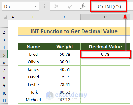
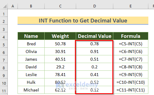
Example 3 – Applying the INT Function to Get a Decimal Value
- Select D5 and enter the following formula.
=C5-INT(C5)Subtracts the output of the INT Function from the decimal number.
- Press ENTER.
- Drag down the Fill Handle to see the result in the rest of the cells.
You will see the decimal values.
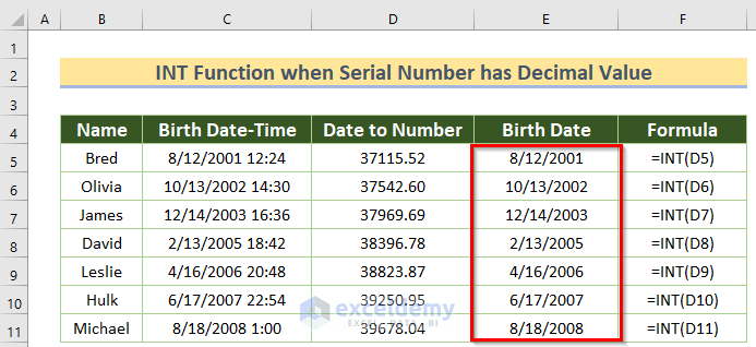
Example 4 – Using the INT Function for Serial Numbers of Decimal Values
The birth date and birth time are provided. To get the birth date excluding the time.
- Select D5 and enter the following formula.
=VALUE(C5)- Press ENTER.
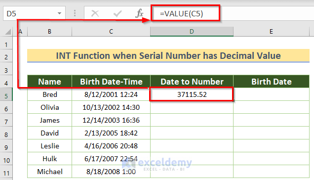
- Drag down the Fill Handle to see the result in the rest of the cells.
- Use the INT formula with the serial number as the argument in E5.
- Press ENTER.
You will get the Birth Date.
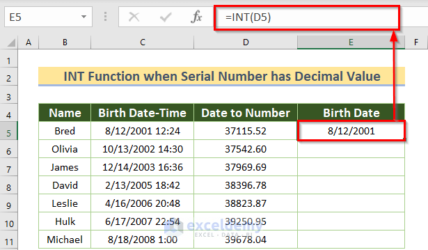
- Drag down the Fill Handle to see the result in the rest of the cells.
You will see all the birth dates.
Example 5 – Using the INT Function to Split Date-Time in Excel
- Enter the formula used in Example 4 to get the birth date.
=INT(C5)- Press ENTER.
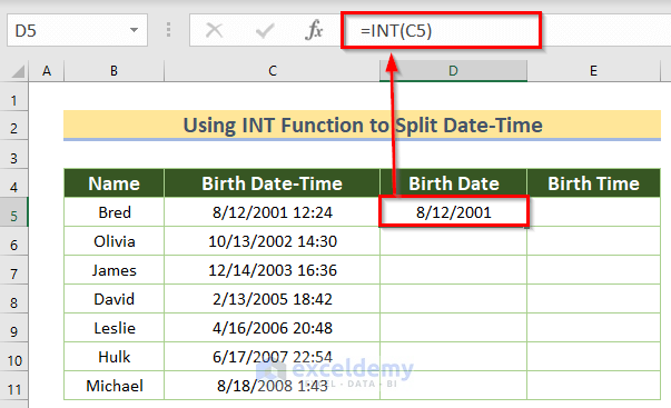
- Drag down the Fill Handle to see the result in the rest of the cells.
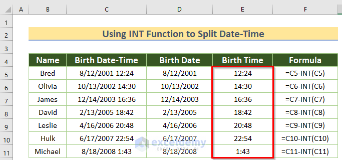
- Use the following formula to get the birth time.
=C5-INT(C5)- Press ENTER.
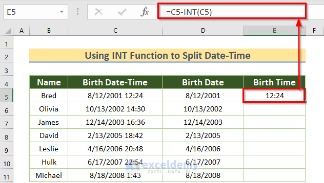
- Drag down the Fill Handle to see the result in the rest of the cells.
You will see all birth times.
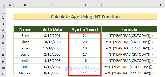
Example 6 – Calculate the Number of Years between Two Dates
Steps:
- Select D5 and enter the following formula.
=INT(YEARFRAC(C5,TODAY()))- Press ENTER.
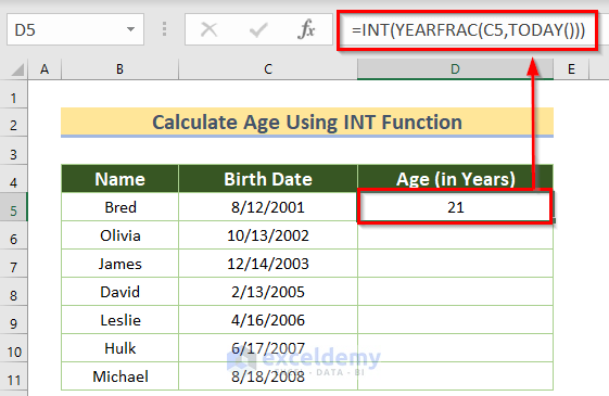
- Drag down the Fill Handle to see the result in the rest of the cells.
You will see all ages in years.
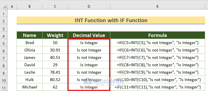
Example 7 – Use the INT Function with the IF Function
To identify integers:
- Select D5 and enter the following formula.
=IF(C5>INT(C5),"Is not Integer", "Is Integer")- Press ENTER.
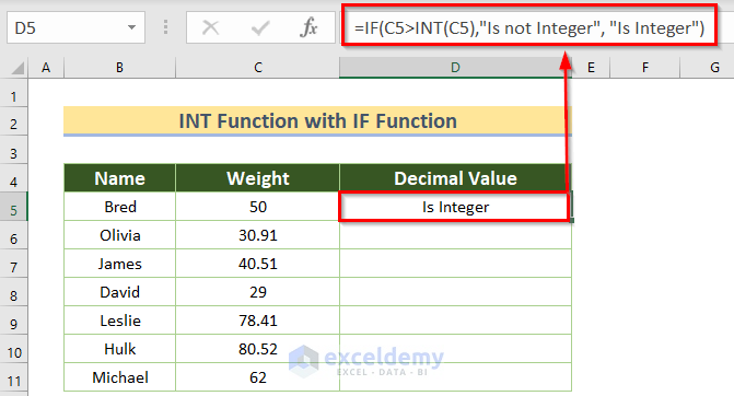
- Drag down the Fill Handle to see the result in the rest of the cells.
You will see all number types.
Example 8 – Applying the INT Function to Round Up Number
To find the weight:
Steps:
- Select a new cell: D5 to keep the result.
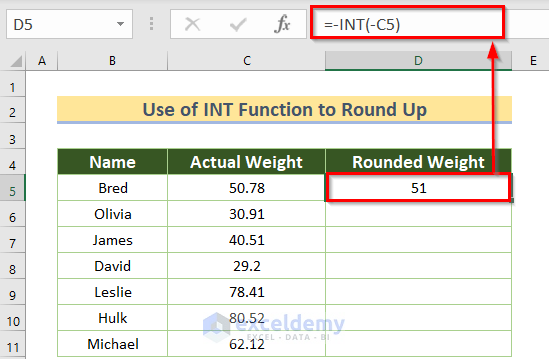
- Use the formula below in D5.
=-INT(-C5)The INT function rounds up the negative numbers. The positive numbers were converted into negative ones using the Minus sign. Use another Minus sign to make the final result positive.
- Press ENTER.
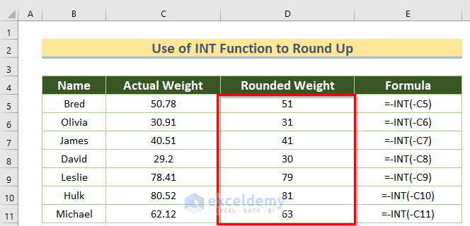
- Drag down the Fill Handle to see the result in the rest of the cells.
You will see the rounded weights.
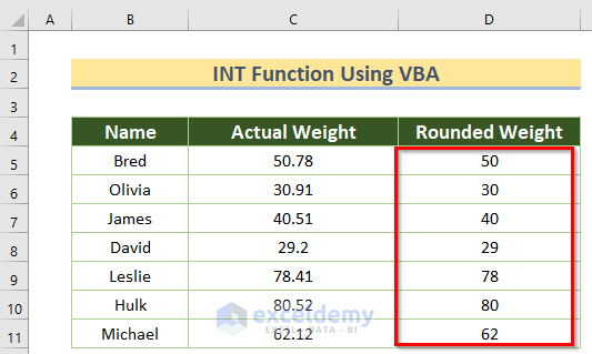
Using VBA with the INT Function in Excel
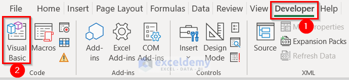
- In the Developer tab > go to Visual Basic.
- Click Insert > Module.
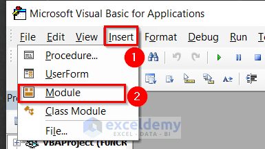
- Enter the following code into the module.
Sub my_example_INT()
Range("D5").Value = Int(Range("C5"))
End Sub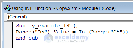
- Save the code and go back to your worksheet.
- In the Developer tab > go to Macros.
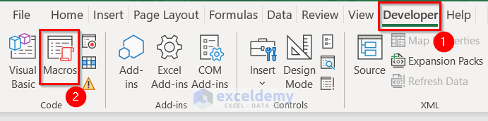
- Run the code by clicking my_example_INT > Run.
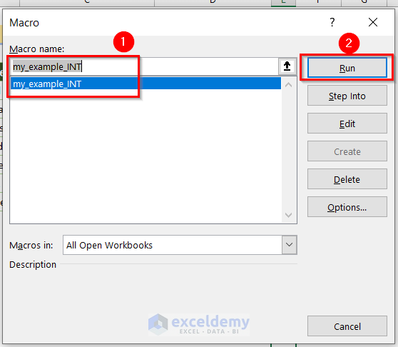
You will see the rounded weight for the value in C5.
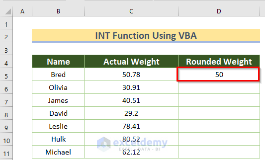
- Apply the same procedure to the other cells.
You will see the rounded weight.
Common Errors While Using the INT Function
| Common Errors | When they show |
|---|---|
| #VALUE! | – a text is inserted as input |
| #REF! | – the input is not valid |
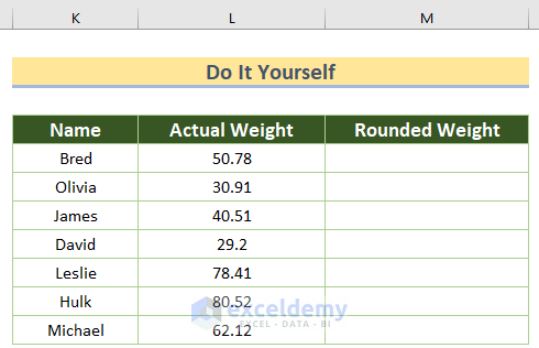
Practice Section
Practice here.
Download Excel Workbook
Download the practice workbook.
<< Go Back to Excel Functions | Learn Excel
Get FREE Advanced Excel Exercises with Solutions!

Hi Abdul,
If it is unacceptable for me to ask for assistance on a problem, I apologize. Otherwise, I would love your input on the problem below.
9/1/22 3/12/18 6:16
9/1/22 13:30
9/1/22 22:43
9/1/22 10:09
4/16/21 8:44
9/1/22 13:11
(Example above)
I have a cell which contains a (reference) date (without a time).
I have a column, each cell of which contains a date & time (various dates and various times). Some of the dates in the column equal the reference date.
I want to find the MAX time, in the column, but only on the reference date. (The times on the other dates don’t matter.)
The solution I’m looking for, in the example, would be 22:43, in cell C3, which is the maximum time on the reference date of 9/1/22.
I’m pretty sure the INT function is involved but I haven’t gotten it to work yet.
Thank you very much, in advance.
Dave
Hello Dave,
Thanks for your humble appearance. But we always welcome informing us about your concerns. Now, without further delay, let’s dive into the problem.
At first, download the Practice Workbook for your own convenience.
From your example above, I’ve created a dataset. Let’s look at the image below for a better understanding.
• To solve the problem, firstly, we are creating a new column named Helper Column to Get Date Only. Also, created a final output range in cell D14.
• Secondly, select cell D7 and enter the following formula.
=DATE(YEAR(B7),MONTH(B7),DAY(B7))This formula filters out the date only from the date and time in cell B7.
• Then, press the ENTER key.
• After that, use the Fill Handle tool to get results in the remaining cells.
• Thirdly, go to cell D14 and paste the formula below.
=MAX(IF(D7:D12=D4,B7:C12))We used the MAX and IF functions in the formula above. Using the IF function, we inserted a logical test that checks if the dates in the D7:D12 range equals to the date in cell D4. If the result is TRUE, then it displays an array of corresponding dates and times in the B7:C12 range. Then, the MAX function gets the maximum value among them.
• As usual, press ENTER.
Currently, it’s showing the time in General format. So, we’ve to change the cell formatting.
• To do this, press CTRL+1 to open the Format Cells dialog box.
• In the Number tab, select Time format as Category.
• Then, choose the formatting Type as shown in the picture below.
• Lastly, click OK.
Finally, we got our desired output format. And the result is correct also.
That’s all about it. If you find any difficulty regarding this example or any other problems related to Excel, feel free to contact us. You can also follow our Exceldemy blog for the most detailed solutions to any problems in Excel.