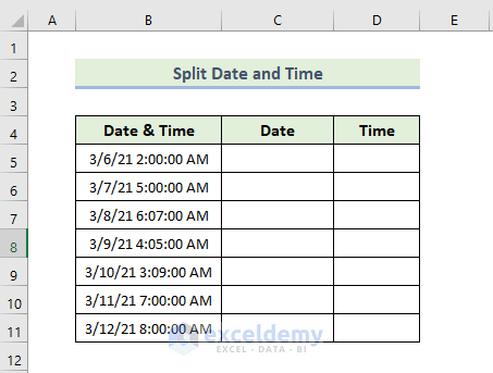
Method 1 – Using the INT Function to Split Date and Time in Excel
We have a dataset containing the date and time. We’ll split them in Columns C and D.
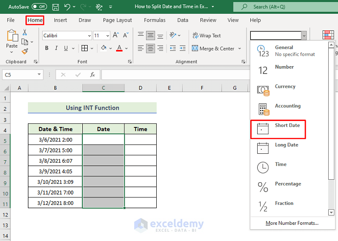
Steps:
- Select the range of cells C5:C11.
- Format them in the Short Date format.
- Use the following formula in cell C5:
=INT(B5)
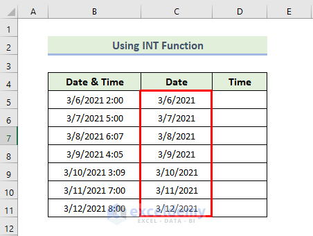
- Press Enter and drag the Fill handle icon down.
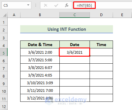
- You will get the date in Column C like the following.
- Use the following formula in the cell D5:
=B5-C5
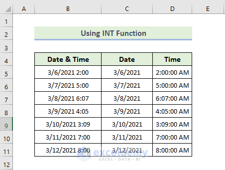
- Press Enter and drag the Fill handle down.
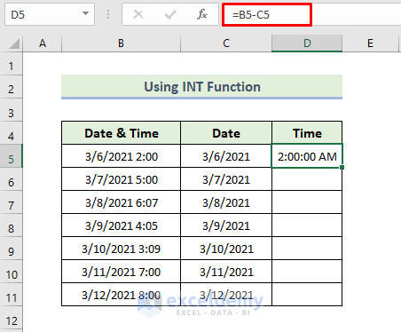
- Here are the results.
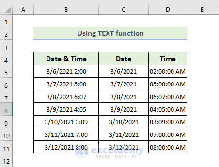
Method 2 – Applying the TEXT Function to Split Date and Time
Steps:
- Use the following formula in cell C5:
=TEXT(B5,"m/d/yyyy")
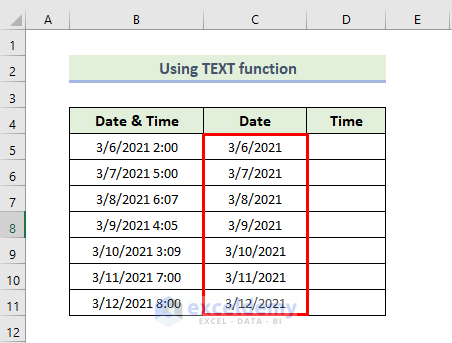
- Press Enter and drag the Fill handle icon down.
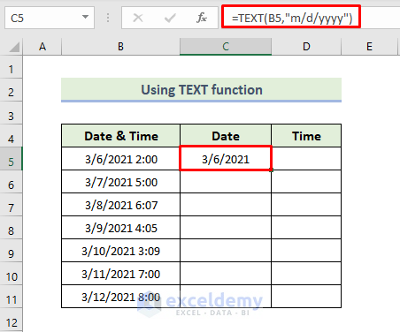
- You will get the date in column C like the following.
- Use the following formula in the cell D5:
=TEXT(B5,"hh:mm:ss AM/PM")
- Press Enter and drag the Fill handle down.
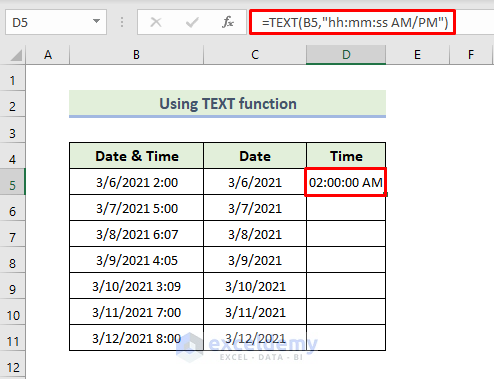
- Here are the split values.
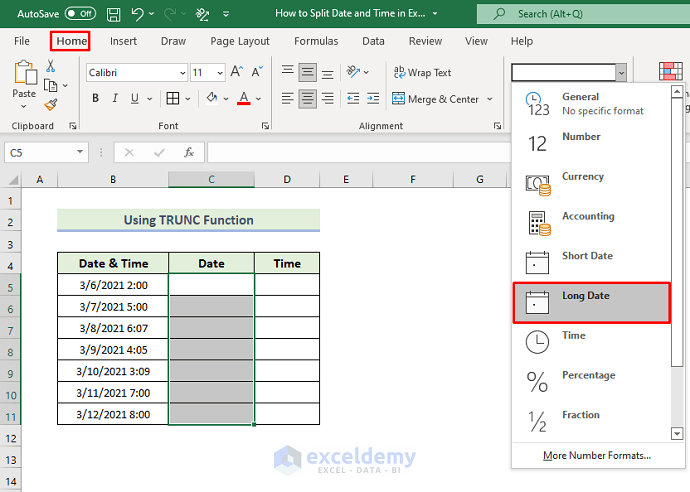
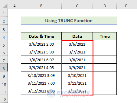
Method 3 – Separating Date and Time with the TRUNC Function in Excel
Steps:
- Select the range of cells C5:C11.
- Format the cells in the Short Date format.
- Use the following formula in cell C5:
=TRUNC(B5)
- Press Enter and drag the Fill handle icon.
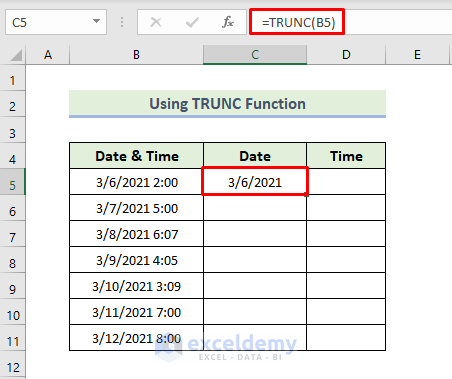
- You will get the date in column C like the following.
- Use the following formula in the cell D5:
=B5-C5
- Press Enter and drag the Fill handle icon.
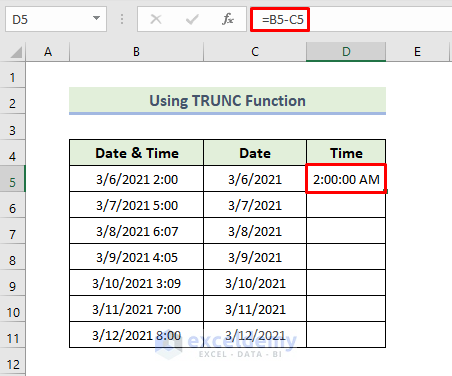
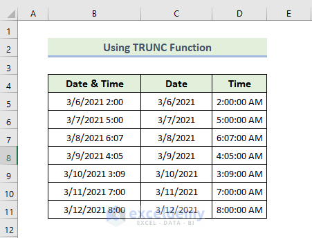
- Here are the split values.
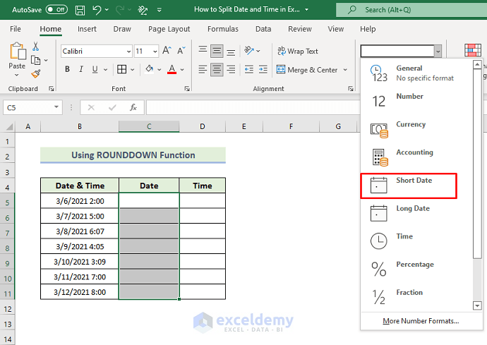
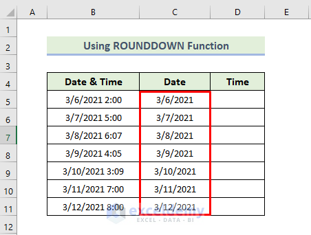
Method 4 – Inserting the ROUNDDOWN Function to Separate Time and Date
Steps:
- Select the range of cells C5:C11.
- Format it in the Short Date format.
- Use the following formula in cell C5:
=ROUNDDOWN(B5,0)
- Press Enter and drag the Fill handle icon down.

- Here’s the result for the date.
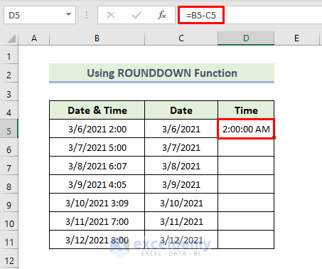
- Use the following formula in cell D5:
=B5-C5
- Press Enter and drag the Fill handle icon down.
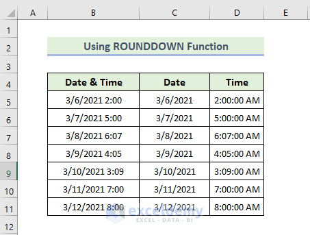
- Here are the split values.
Method 5 – Separating Date and Time with the Flash Fill Tool
Steps:
- Type the first two dates in C5 and C6.
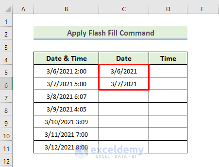
- Go to the Data tab, select Data Tools, and select the Flash Fill option.
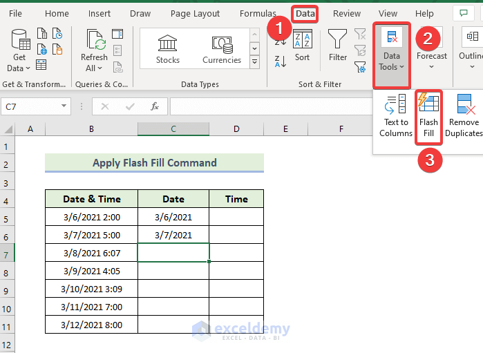
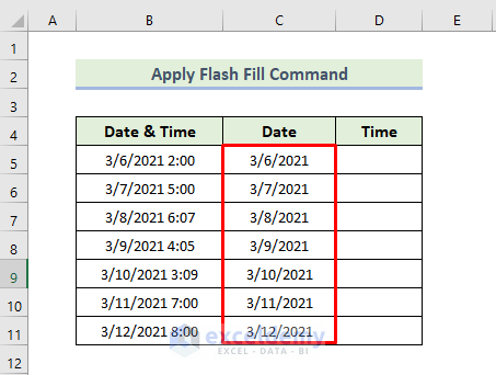
- You will get the date in column C.
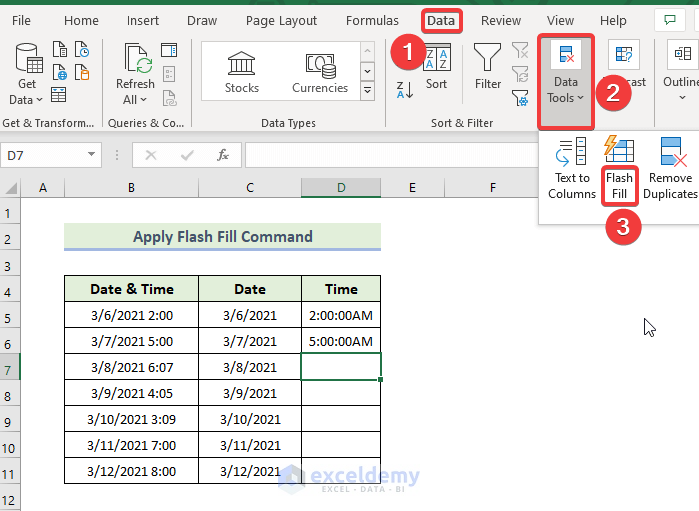
- Type the first two times in D5 and D6.
- Go to the Data tab, select Data Tools, and select the Flash Fill option.
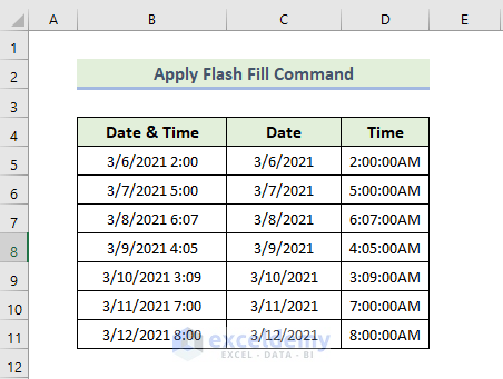
- Here are the results.
Method 6 – Splitting Date and Time Through a Keyboard Shortcut
Steps:
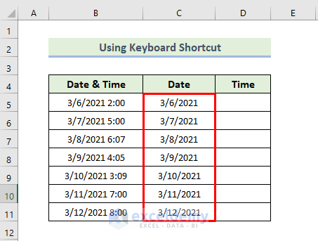
- Type the first two dates in C5 and C6.
- Press Ctrl + E.
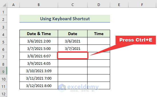
- You will get the date in Column C.
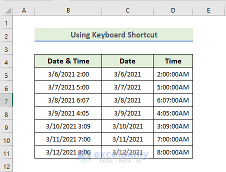
- Type the first two times in D5 and D6, and press Ctrl + E.
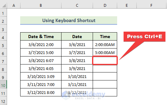
- You’ll get the split values.
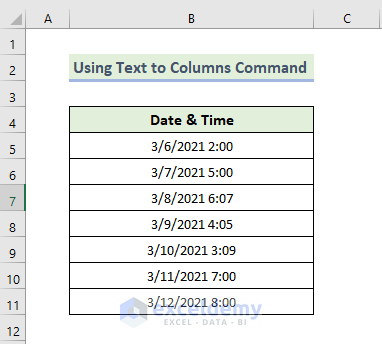
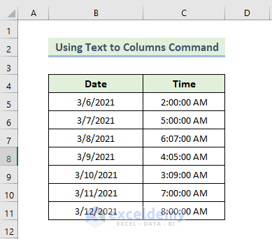
Method 7 – Using the Text to Columns Tool to Split Date and Time
We have a dataset containing the date and time.
Steps:
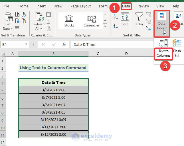
- Select the range of the dataset.
- Go to the Data tab, select Data Tools, and choose the Text to Columns option.
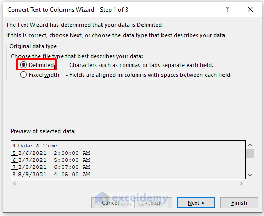
- When the Convert Text to Columns Wizard – Step 1 of 3 dialog box appears, check the Delimited option.
- Click on Next.
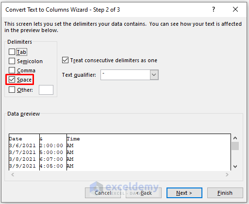
- The Convert Text to Columns Wizard – Step 2 of 3 dialog box appears.
- In the Delimiters section, check Space.
- Click on Next.
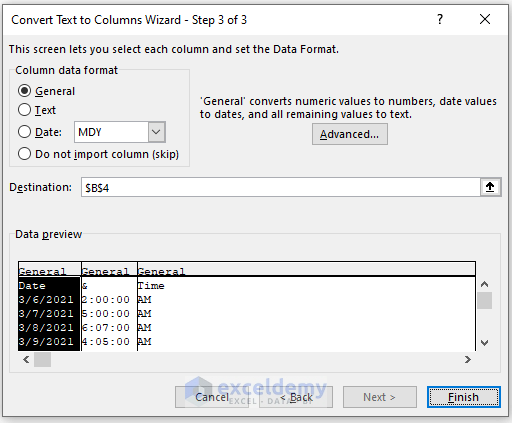
- The Convert Text to Columns Wizard -Step 3 of 3 dialog box appears. Click on Finish.
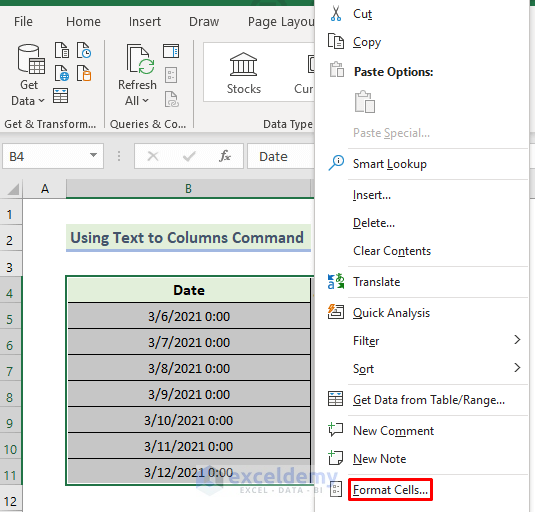
- You will get the date in column B like the following and you need to customize the date. Select the range of the cells, right-click, and select the Format Cells option.
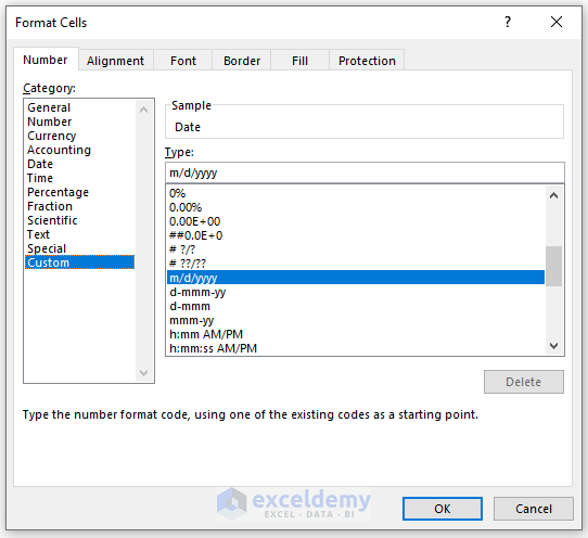
- When the Format Cells dialogue box appears, select Custom from the Category.
- Select your desired date type from the Type section.
- You will get the date in column B like the following.
- Select the range of the cell of column Time. Go to the Home tab and select the Time format.
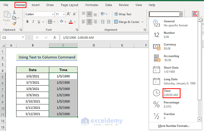
- Here are the split values.
Method 8 – Splitting Date and Time with Excel Power Query
Steps:
- Select the range of the dataset.
- Go to the Data tab and select From Table/Range.
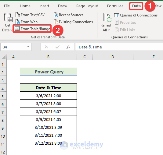
- You can see your dataset in Power Query Editor.
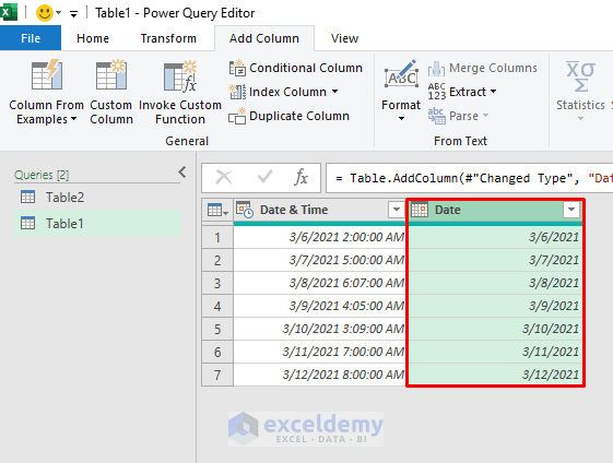
- Go to the Add Column tab, select Date, and choose the Date Only option.
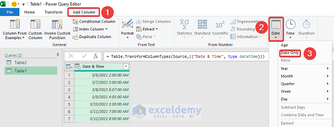
- You will get a new column with dates.
- Select the range of the original dataset.
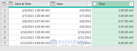
- Go to the Add Column tab, select Time, and choose the Time Only option.
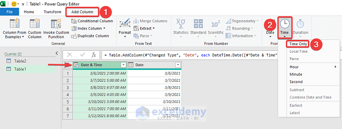
- You will get a new Column with times.
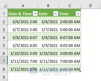
- Go to the Home tab and select Close & Load.
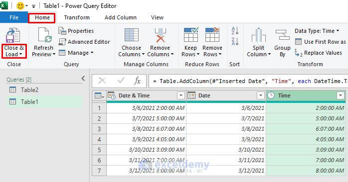
- You’ll get a new sheet with the split values.
Download the Practice Workbook
Split Date and Time: Knowledge Hub
<< Go Back to Split | Learn Excel
Get FREE Advanced Excel Exercises with Solutions!
