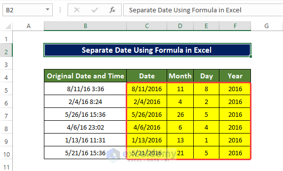
How to Separate Date in Excel Using Formulas (5 Methods)

Dataset Overview

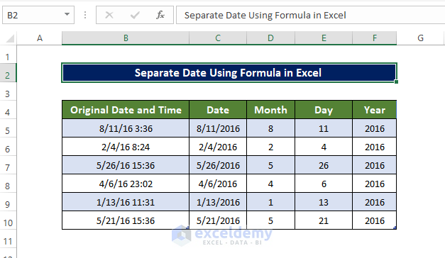
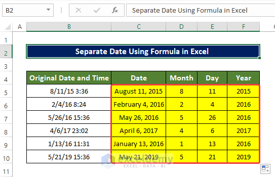
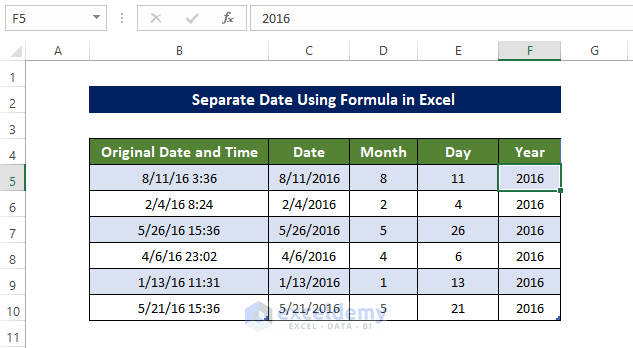
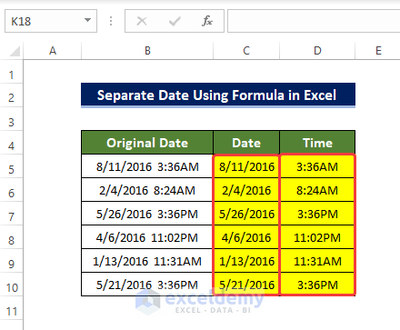
For this demonstration, we’ll be utilizing the dataset provided below. In the range of cells from B5 to B10 on the left, you’ll find the Original Date and Time column, which combines both the date and time. In the adjacent columns labeled Date, Month, Day, and Year, we have separated out the individual date components. We will discuss in detail how to extract these values from the Original Date and Time column.

Method 1 – Using TEXT Function to Separate Date

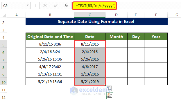
Select cell C5.
Enter the following formula to extract the date from the combined date and time in cell B5:

=TEXT(B5,"m/d/yyyy")

- This formula will display only the date portion in cell C5.

Drag the Fill Handle down to cell C10. Now the range of cells C5:C10 will be filled with dates extracted from the range of cells B5:B10.

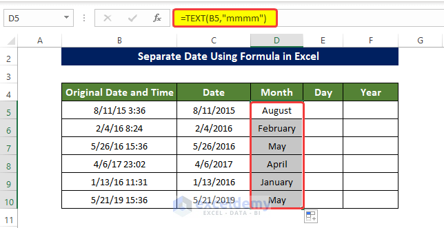
To extract the month from the date, select cell D5 and enter the formula:

=TEXT(B5,"mmmm")

- This will show only the month part of the date in cell D5.

Drag the Fill Handle down to cell D10 to fill the range of cells D5:D10 with months from the original date and time data.

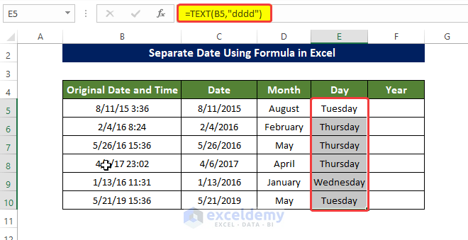
For extracting the Day, select cell E5 and enter the formula:

=TEXT(B5,"dddd")

- Cell E5 will display only the day part of the date and time.

Drag the Fill Handle down to cell E10 to populate the range of cells E5:E10 with days from the original data.

To extract the year, select cell F5 and enter the formula:

=TEXT(B5,"yyyy")

- Cell F5 will show only the year part of the date and time.

Drag the Fill Handle down to cell F10 to complete the extraction of years from the original data.

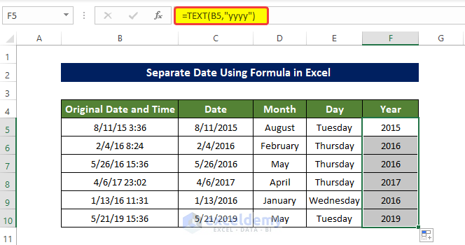
And that’s how you can separate date, day, month, and year from a combination of date and time using the TEXT function in Excel.

Method 2 – Utilizing DATE Function in Excel

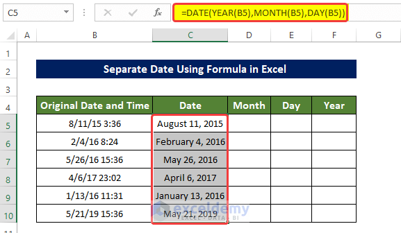
Select cell C5.
Enter the following formula to extract the date from the combined date and time in cell B5:

=DATE(YEAR(B5),MONTH(B5),DAY(B5))

- This formula will display only the date portion in cell C5.

Drag the Fill Handle down to cell C10. Now the range of cells C5:C10 will be filled with dates extracted from the range of cells B5:B10.

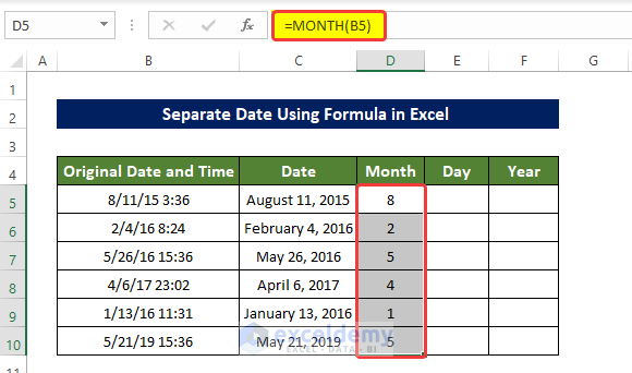
To extract the month from the date, we’ll use the MONTH function. Select cell D5 and enter the formula:

=MONTH(B5)

- This will show only the month number of the date in cell D5.

Drag the Fill Handle down to cell D10 to fill the range of cells D5:D10 with month numbers from the original date and time data.

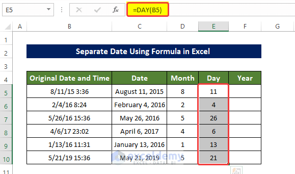
For extracting the day, we’ll use the DAY function. Select cell E5 and enter the formula:

=DAY(B5)

- Cell E5 will display only the day part of the date and time.

Drag the Fill Handle down to cell E10 to populate the range of cells E5:E10 with days from the original data.

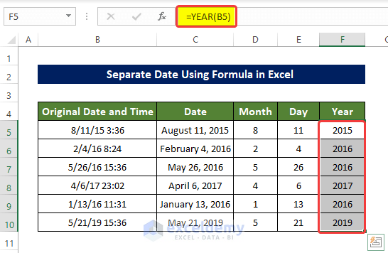
To extract the year, we’ll use the YEAR function. Select cell F5 and enter the formula:

=YEAR(B5)

- Cell F5 will show only the year part of the date.

Drag the Fill Handle down to cell F10 to complete the extraction of years from the original data.

And that’s how you can separate date, day, month, and year from a combination of date and time using the DATE function in Excel.

Method 3 – Separating Dates Using the INT Function in Excel

Select cell C5.
Enter the following formula to extract the date part from the combined date and time in cell B5:

=INT(B5)

- This formula treats the combined value as a whole number, separating the integer part as the date.

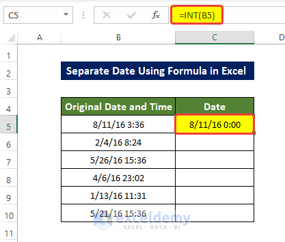
Drag the Fill Handle down to cell C10. The range of cells C5:C10 will be filled with dates extracted from the range of cells B5:B10.
However, if you look carefully, there is still time formatting showing in the range of cells C5:C10, even though they display a null (zero) value.

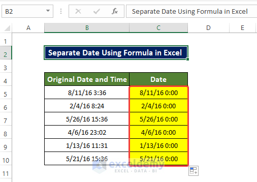
To resolve this issue, we need to change the format of the range of cells C5:C10 from General to Short Date format.
To do this:
- Select the range of cells C5:C10.
- Go to the cell format option from the Number group in the Home tab.
- Click the button, and a drop-down menu will appear.
- From that menu, select Short Date.

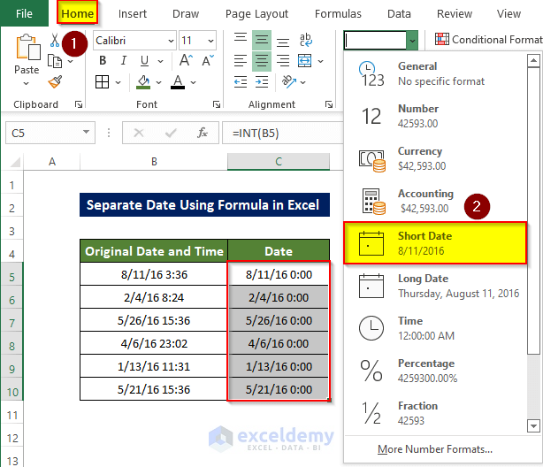
After clicking Short Date, you will see that all the dates now have only the date format without any time information.

And that’s how you can separate the date portion from a combination of date and time using the INT function in Excel.

Method 4 – Using TRUNC Function to Separate Date in Excel

Select cell C5.
Enter the following formula to extract the date part from the combined date and time in cell B5:

=TRUNC(B5)

- This formula truncates the fractional part of the number, treating it as a whole number representing the date.

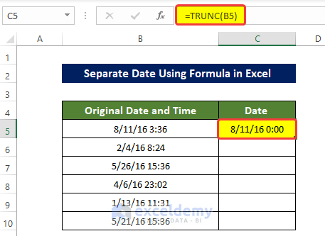
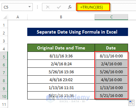
Drag the Fill Handle down to cell C10. Now the range of cells C5:C10 will be filled with dates extracted from the range of cells B5:B10.
However, if you look carefully, there is still time formatting showing in the range of cells C5:C10, even though they display null (zero) values.

To resolve this issue, we need to change the format of the range of cells C5:C10 from General to Short Date format.
To do this:
- Select the range of cells C5:C10.
- Go to the cell format option from the Number group in the Home tab.
- Click the button, and a drop-down menu will appear.
- From that menu, select Short Date.

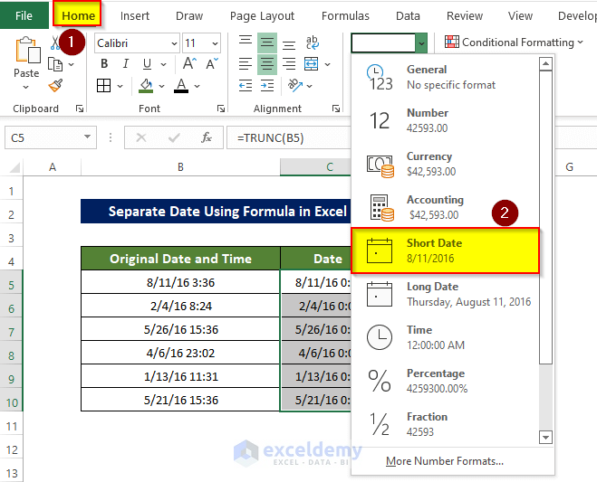
After clicking Short Date, you will see that all the dates now have only the date format without any time information.

And that’s how you can separate the date from the combination of date and time using the TRUNC function in Excel.

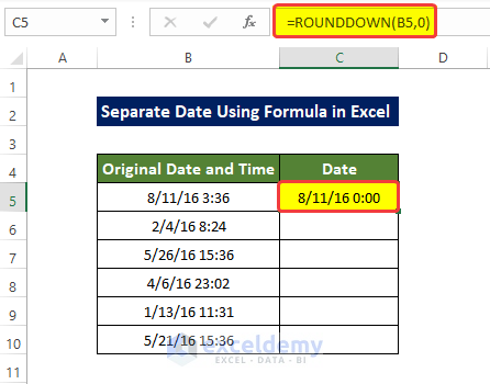
Method 5 – Utilizing ROUNDDOWN Function

Select cell C5.
Enter the following formula to extract the date part from the combined date and time in cell B5:

=ROUNDDOWN(B5,0)

- This formula will round down the number to the nearest integer, effectively treating it as a whole number representing the date.

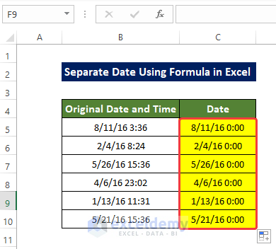
Drag the Fill Handle down to cell C10. Now the range of cells C5:C10 will be filled with dates extracted from the range of cells B5:B10.
However, if you look carefully, there is still time formatting showing in the range of cells C5:C10, even though they display null (zero) values.

To resolve this issue, we need to change the format of the range of cells C5:C10 from General to Short Date format.
To do this:
- Select the range of cells C5:C10.
- Go to the cell format option from the Number group in the Home tab.
- Click the button, and a drop-down menu will appear.
- From that menu, select Short Date.

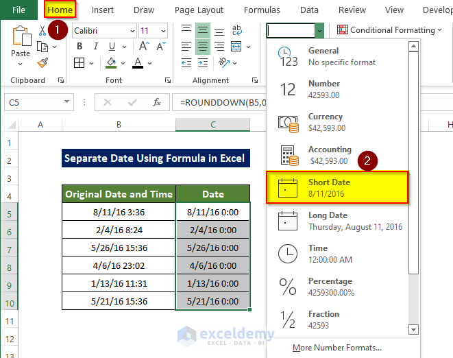
After clicking Short Date, you will see that all the dates now have only the date format without any time information.

And that’s how you can separate the date from the combination of date and time using the ROUNDDOWN function in Excel.

3 Alternative Methods to Separate the Date without a Formula in Excel

Method 1 – Separating Dates Using Power Query

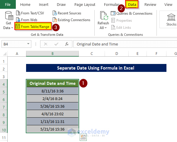
Select the range of cells (B4:B10) that contain the dates you want to separate.
Go to the Data tab and find the Get & Transform Data group.
Click on From Table/Range.

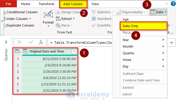
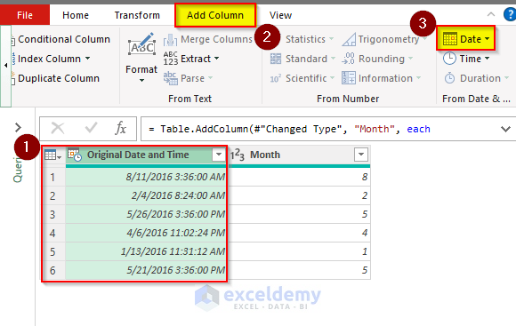
In the new window, go to the Add Column tab. Under the From Date & Time group, select the Date command. Choose Date only from the drop-down menu.

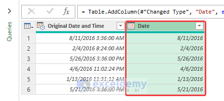
- This will create a new column with only the dates.

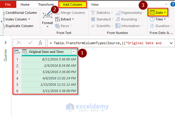
- Repeat the process for the month. Under From Date & Time, select the Date command.

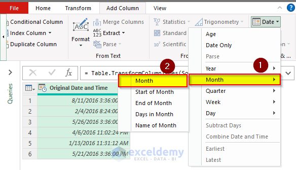
- Choose Month and select Month from the drop-down menu.

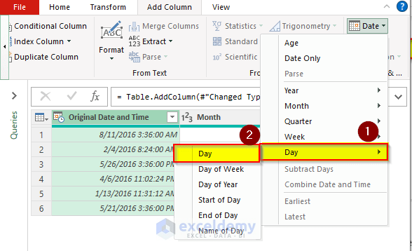
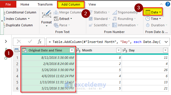
- Create a new column for the day.

- Use the Date command and select Day.

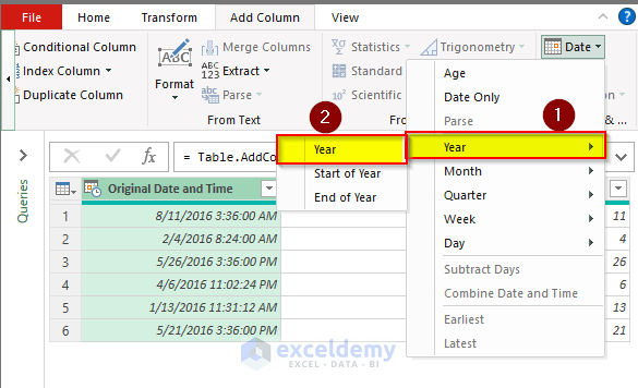
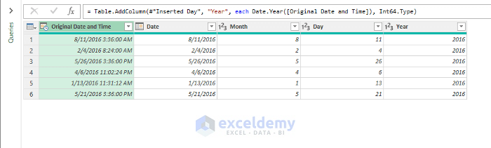
- Create a column for the year.

Use the Date command and choose Year and select Year.

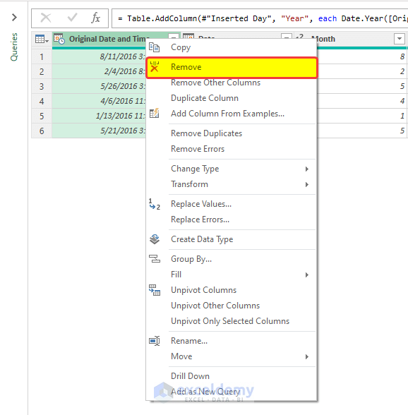
Right-click on the original date and time column and select Remove from the context menu.

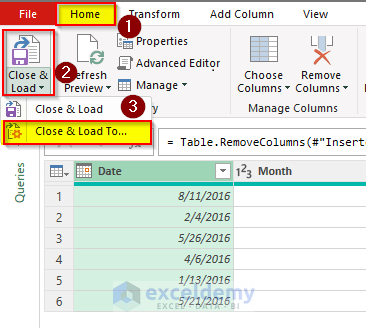
Go to the Home tab and click on the Close and Load icon. Choose where you want to load the result (e.g., a new worksheet).

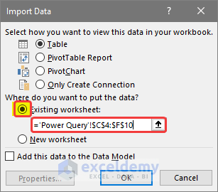
A new window named Import Data will open, from that window, choose Existing worksheet from Where do you want to put the data? option.
After that choose the location of the new columns. In this case, we select $C$4:$F$10. Click OK.

You will notice that the column is loaded next to the original dataset. And it contains the dates, days, months, and years of the original dataset.

Method 2 – Utilizing Text to Columns to Separate Dates

Begin by selecting the range of cells (B5:B10) that contain the combined date and time values.
Go to the Data tab and click on the Text to Columns icon.

In the new window, select the Delimited option and click OK.

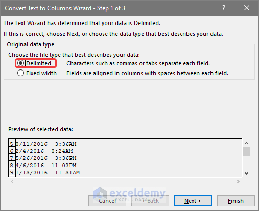
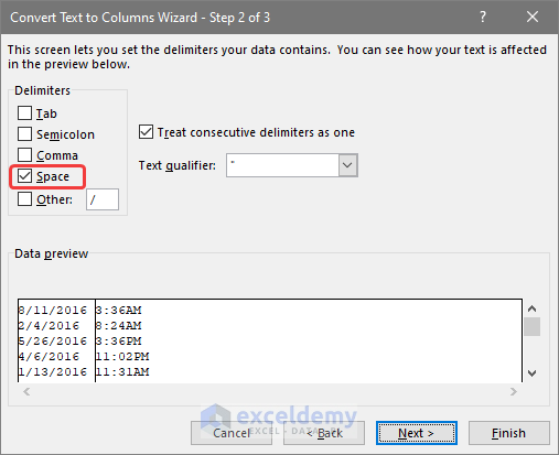
- In the next window, mark only the Space option under the Delimiters group and click Next.

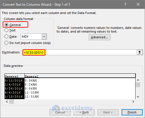
Choose General under the Column data format group.
Specify the destination location for the separated values (e.g., $C$5:$D$10).

A preview below the destination box will show how the data will look after separation.
Click Finish to complete the process.

After following these steps, you’ll notice that the dates are now separated from the time in the range of cells C5:C10.

Method 3 – Using Flash Fill to Separate Dates in Excel

Start by selecting cell C5.
Enter the date exactly as mentioned in cell B5.

Drag the Fill Handle icon (located at the bottom right corner of the cell) while right clicking the mouse to cell C10.
From the Context Menu, select Flash Fill.

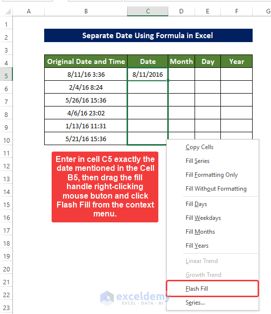
- The range of cells C5:C10 will now contain only dates.

In cell D5, enter the month number from cell B5.
Drag the Fill Handle to cell D10.
Again, select Flash Fill from the Context Menu.

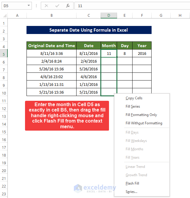
The range of cells C5:C10 will now display only the month numbers.
Enter the day exactly as mentioned in cell E5.
Drag the Fill Handle to cell E10.
Then select Flash Fill from the Context Menu.

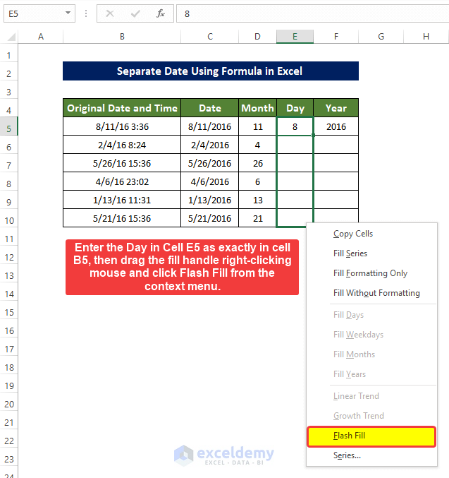
The range of cells C5:C10 will now display only the day numbers.
Enter exactly the year number of cell B5 in cell F5. Drag the Fill Handle to cell F10.
Select Flash Fill from the context menu.

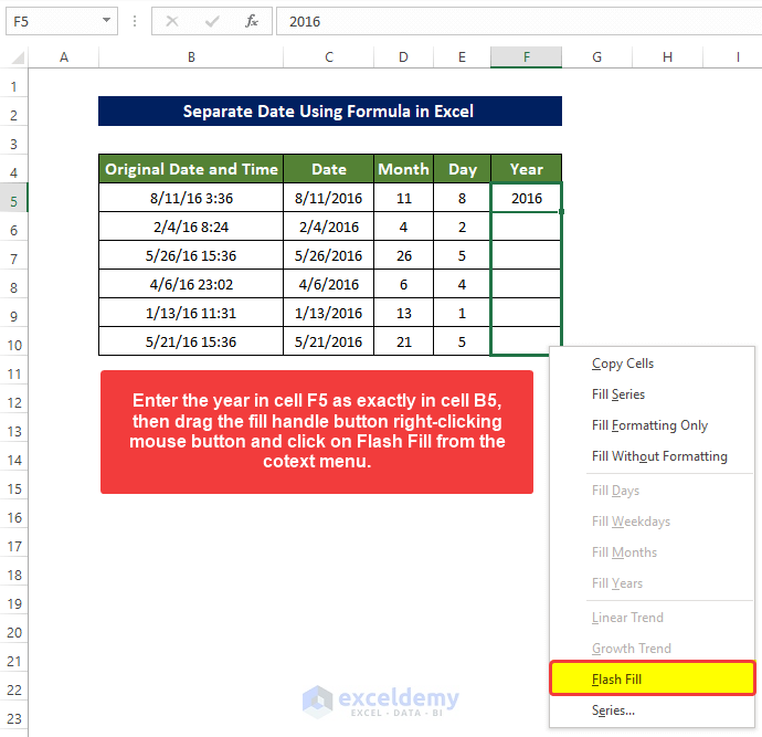
After completing these steps, the range of cells C5:C10 will have separate columns for dates, months, days, and years, effectively separating the date from the original combined date and time in the Excel worksheet.