Latest Posts From Rubayed Razib Suprov
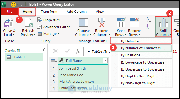
In this article, we are going to see how we can split columns in Excel using various methods. In Excel, we need to split columns on many occasions. Sometimes ...

Here's an example where we presented a sample funnel chart that was created with the help of a previously created stacked chart. How to Create a ...

This is an overview: Download Practice Workbook Download the practice workbook. VLOOKUP.xlsx Solution 1 - The Lookup Value ...

In Microsoft Excel, the TextBox control is a powerful feature that facilitates seamless text and numeric data entry, enhancing user interaction within ...

Below, you can see how the watch window monitors the variable value in Excel VBA. How to Add a Watch Window Open the VBA code editor window. ...

In this article, we will show you how to use Excel to compare sheets side by side. Comparing various datasets at the same time is a very common scenario in our ...

The Array Function is a very useful tool in Excel to store data and limit the use of the variable, which is basically saving a lot of memory usage of the ...

In this article, we will demonstrate how to use the Exit Do command inside the Do While loop. The Exit Do command inside the Do While enables us to escape the ...

Not only in VBA, the If-Else-if condition is a widely popular conditional tool to investigate the conditions and then carry out tasks. This effective command ...

Method 1 - Filter a Pivot Table Based on Single Criteria Using VBA STEPS: To create a pivot table, a sample code is given below. The ...

Method 1 - Using Call Function Using the Call Function we can call a sub and execute the task inside the sub directly. There are three ...

Here's a sample example of using the correlation coefficient to analyze data. Download the Practice Workbook Download this practice workbook ...

To demonstrate how to assign a macro to a button, we'll use a simple dataset containing student information. We'll sort this data according to the age of the ...
Example 1 - Use the Intersection Command and a Function Button in Excel Steps: Press F9. Enter the first level of rows, here C5:E7. Enter a space ...

Overview of a 2-Dimensional Array (2D Array) Definition A 2-dimensional array, also known as a 2D array, is an array that has data spread out in two ...
- 1
- 2
- 3
- …
- 10
- Next Page »
See Our Reviews at


Thanks for your question. Actually, you can approach this problem in two separate ways. One is directly calculating the significant value or using a chart. For the chart, you need to calculate the T value first, and then you will calculate the p-value. Using them, you can calculate the critical value from a chart available online.
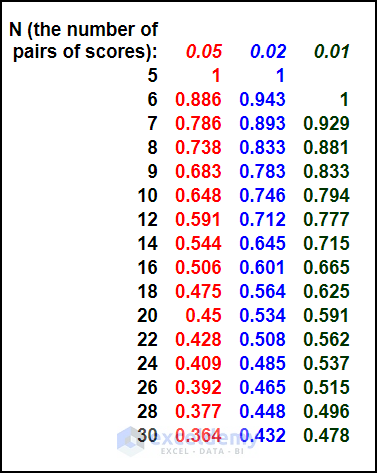
1. The formula for calculating the T value is, t=r_s×√((n-2)/(1-r_s^2 ))
Where r_s is the Spearman correlation value.
n is the no of entry
The Excel formula would be in our case =E17*SQRT((E16-2)/(1-E17^2))
2. The formula for significant value, p =T.DIST.2T(ABS(calculated t value),n-2)
3. To calculate the critical value, you need to have a critical value chart. Using the p-value and the n (Number of entries), from the chart, you need to get the critical value.
4. You may be needed to interpolate the critical values as you may not have the exact p or n values. If your correlation value>critical value, then there is a significant correlation between the values. In other words, the correlation result is significant.
Thanks for your question in our platform.
You may opt for the first method mentioned here to prevent Excel sheet content to another workbook completely.
Or you can read the article(https://www.exceldemy.com/protect-excel-sheet-from-copy-paste/#1_Use_Info_Option_to_Protect_Excel_Sheet_from_Copy-Paste) to prevent the workbook content from being copied to another workbook. You can ignore the VBA coding method if you want.
Use the following formula =IFERROR(VLOOKUP(B5,D5:E9,2,FALSE),””)
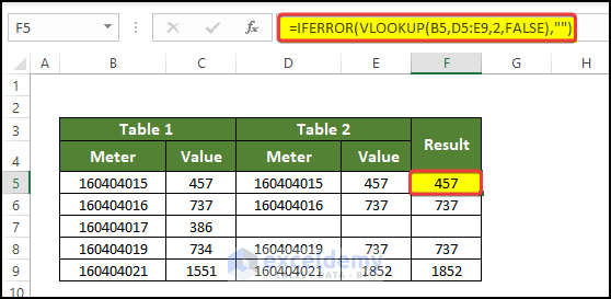
Your given sample table is stored in column B: D. And this VLOOKUP function will look for the value of cell B5(table 1) in the first column on table 2, and then using that position, will return the meter reading from the E column. And it will return blank if there isn’t any meter reading.
The RAND function is supposed to return only a random value, which is used for shuffling the dataset values. In this case, we are trying to swap cell values within two separate cells. This means your statement is not applicable. If you insist that it is possible, please write down the process or send us your Excel file through email. Thank you.
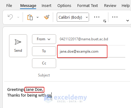
Greetings Gin Got,
Sorry for the issue that you are facing. Unfortunately, the issue of 255 characters in a single cell is a fundamental feature in the Excel environment. But on the other hand, the character limit in a formula is infinite. So I suggest you stick to this article’s first or second method.
Now coming to the 4th method in which you are not getting so much success, is that this method is only for Users of Excel 2007-Excel 2013 in a very specific area. Users who are getting trouble importing data to the Myssql server are experiencing this issue of getting characters truncated in the cell. This 4th method is the solution for that reason. The article will now be updated with a note with this disclaimer. If you need further assistance then please feel free to contact us again, attaching necessary files is recommended.
Thanks and Regads
Rubayed Razib
You an find the solution in the below comment of yours. I have provided a reply with a code and explanation image.
Greetings Valerie,
Sorry to hear about your inconvenience. Actually from our side, we are not facing issues while moving the rows. It is working quite well. If you are incorporating this code with another code there might be an issue in the parent dataset or in the sheet name. It will be much easier for us to assist you if you can provide us with your sample code, doing so we can have a look inside the code and try to identify the issue.
Still for your convenience, we are attaching another code, you can take a look and try y yourself. You need to change the sheets name(source and the destination) and the search value alongside the seourcerange(in which column you want to search the values).
Greetings Chalon,
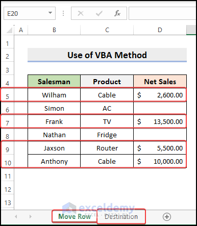
Below I am going to provide a code using which you will be able to move only the rows that have value in the corresponding cells in a specific column. The sheet name here termed as “Destination” and the sheet from where we want to move the cell are named as “Source”. After putting the code in the code editor, press the Run command buton.
After running the code,we will see that the rows corresponding to the cell values are now mooved to the destination sheet.
Greetings Vinod,
The code provided above is actually working quite well for multiple members of our team. The Error you experienced is local and I advise you to review the code and check whether you made any altercation to the code. Try to paste the code as given here same to the editor. Just change the attachment address according to your need.
The specific error that you are experiencing might be the cause of using the same variable k in multiple places. Again, in our code, we did not use the variable in multiple places in the same code. Try to paste the same code that we provided or change the variable name to something else, like K1. Hope this helps.
Thanks and Regards
Rubayed Razib
Team Exceldemy
Greetings Prasanth,
Thanks a lot for the question you asked. Below I provide a code using which you can add rows in another worksheet. When you run the code, then you will see that the values stored in the C3:D3 insert in another worksheet. The values are now repeated according to the value mentioned in the cell E3
Greetings Edward,
Thanks a lot for your Question in our blog post. Now the issue you have is a little bit unclear to me. Can you provide a sample output manually which will contain your desired result? In that way, your problem be more clear to us and in turn it will help us to resolve your problem.
Greetings Prasanth,
Thanks a lot for your question. You can follow the modified code given below to insert rows to another sheet.Here the input tanges are in the Sheet1 and the Output ranges where the rows are going to be inserted Sheet2.
Greetings Pooja,
You might want to know how you can attach a whole dataset to the worksheet. For this, you can follow this article from our website. In this article, you will know how you can attach values to the worksheet from the inputbox values. If your query is related to something else, please elaborate on your problem with examples.
Greetings Beck,
Thanks a lot for your question. I am not entirely sure if your question is pertinent to topic of the this article, or if it is just a standalone question. I am giving you a response treating the question as a standalone question.
To have different values in the cell which is 10 digits long and starts with 430, paste the below code in the code editor, and then press Run.
After pressing Run, you will notice that the code now put 10 distinct 10-digit values in the worksheet starting with 430.
Hope this helps, if you have any other question or suggestions,please do not hesitate to comment on this post.
Greetings,
I understand your query. You asked about attendence sheet for both monthly and weekly basis. But my suggestion will be to go on with the monthly basis assesment. In this way your job will be much smoother. Secondly I provided a demo sheet that actually contains the attendence with time picker drop down, and summation of total hour of work in a month.The time picker need to have a fixed time and they are specified below the sheet.You just need to enter the month and year in the beginning and then you can enter the in time and out time using the time picker.
The download file can be accessed from the link below,
https://www.exceldemy.com/wp-content/uploads/2023/04/Attendence-SheetMonthly.xlsx
Thanks a lot for posting your query in Exceldemy
Below I am giving you a VBA code using which you can open the outlook template saved on your pc and then replace them with desired text from the Excel sheet.
the sample template file that we are using is given below.

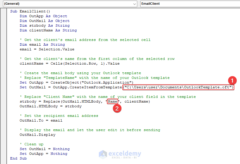
The Name, in the beginning, is going to be replaced by the desired name and the recipient will be the selected mail address.
In the code, two separate things must be taken seriously, firstly the location of the template file. The location of the template mail has to be specified correctly in the code(Marked as 1), as shown in the image. So please rewrite the location of the file correctly.
secondly, f you need to specify which term to replace with names inside the code(Marked as 2).
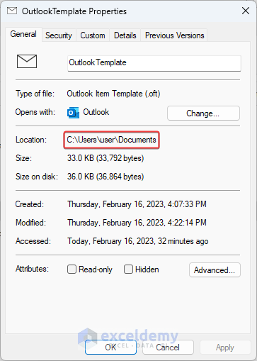
the location of the template file in your pc can be found in the properties tab as shown below.
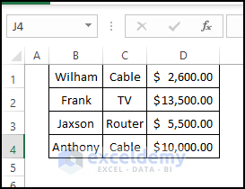
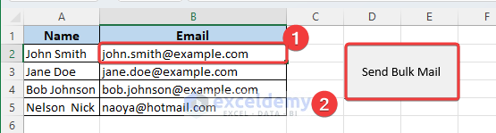
finally, you are ready to execute the code.For this, you have to first select the email address to which you want to send the email. Then Run the Macro by pressing the Macro button placed just right side of the information.
Then you can see that the a new email has been composed with the name placed in the beginning with the selected mail address as the recipient.
You can download the sample macro file from the links below
Sample Macro File: https://www.exceldemy.com/wp-content/uploads/2023/02/Send-Automatic-Email-outlook-template.xlsm\
In case you need to template file, please contact us through email.
Regards,
Rubayed Razib
Thanks a lot Salih, for your query
I think I understood your problem. Here, your cant put the table name in this way. You have to insert the table name in between two apostrophe symbol. So basically your code line should be like
Set t = x.ListObjects(“Depart_Filter5”)
Thanks a lot for your response John,
Here there might be some other issues underlying your file that is causing issue for you. It would be better if your share your file with us and we can have a look into it.
Thanks a lot for your appreciation.
Greetings TRISH,
In your case, it is difficult to ans this problem without having a look at your worksheet . Please send the worksheet to our problem solving, hence we can assist you on this issue.
Greetings Debbie,
First of all,we really appreciate for your question. Now if I am not afraid, you asked about why your total percentage value not changed despite deleting one sample value. If this is the case, the reason is pretty simple. as you delete one value, your total value also change. Which in turns also change the percentage value of all the other values. and this change will happen in a way that the total percentage values are always sums up to 100, following the basic arithmatic rule.
If this is not the case,please provide your Excel worksheet containing your data and we will have a look.
Thanks and Regards
Rubayed Razib
Greetings Rob,
Thanks a lot for commenting on this article. Unfortunately, we managed to find only the last three companies and the INVESTEC CORE FUND IWCF among the companies you metioned in the database. Rest of them are not enlisted in the database. I have given the dataset link containing the stock informations of the Satrix RESI ETF SATRIXRESI, Coronation Global Capital Plus [ZAR] Feeder CPLSZ, Ninety One Equity Fund NINEQ, INVESTEC CORE FUND IWCF etc.
Thanks and Regards
Rubayed Razib
Dataset Link:https://www.exceldemy.com/wp-content/uploads/2023/01/Get-Stock-Prices-in-Excel.xlsx
Thanks a lot for providing the correction. Both the Image and the Formula has been updated.
Hello Amghar,
Thanks a lot for submitting Excel related problem at Exceldemy. Here you can use the VBA code mentioned below.
In that code, you need to mention the cell address inside the VBA code range property(as shown in the image). After this, if the condition satisfied, the cell row height will adjust accordingly.
Thanks a lot for submitting question in Exceldemy. From our end, every single method is actually working perfectly. Could you please specify which method you are experiencing this error with? Did you test with the dataset provided here? If not, could you please send us the Excel files?
Thanks a lot for your compliments, Raul. Glad to hear that the article came in handy for you
Thanks a lot for your comment, we will take your suggestions into consideration in the future.
Thanks for your question. Here Seattle has a rating of -0.50409…And St Louis Rams has -4.439784. if you subtract -0.50409 from the -4.439784, then you will get 4.943874.which is approximately around 4. So the statement that “Seattle has 4 points better than St Louis”
Thanks a lot for your appreciation.
Thanks a lot for your question. In the screenshot, all of the P values are actually below 0.05. One value is 0.002384973 and another one is 1.4769*10^-10. Maybe you got a little confused as the letter E is hard to notice. Hope this helps.
Thanks for your question, Jorge F. The allocation of memory mostly depends upon the dataset in which you are working on, and how they are interacting to other functions. For example, if you use a nested function, that function will cost more memory. There are some functions out there that consume more memory compared to other functions. Among the methods described above, the SUMPRODUCT function has more memory allocation compared to other functions. The other two methods would consume more or less the same amount of memory.
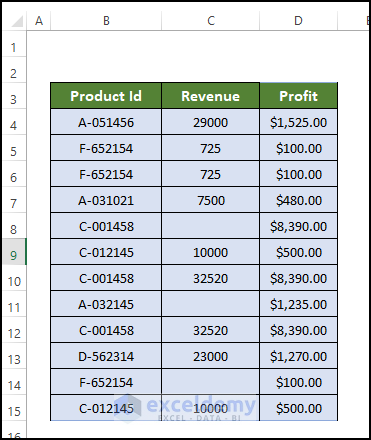
Thanks a lot for your question, Aaron. Here we are going to use a separate formula for highlighting the entire row based on whether any of the values in the row are blank or not. Notice the image below, we got blank cell in C8,C11, and C14
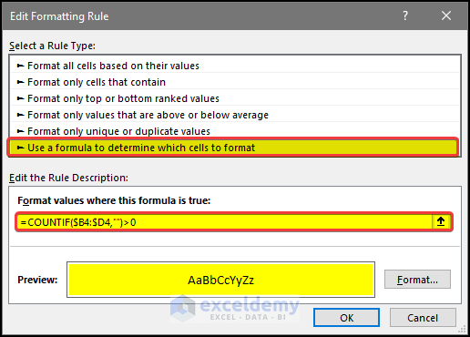
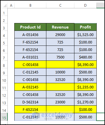
2. First, go to the Conditional Formatting, and set the rules as shown below.
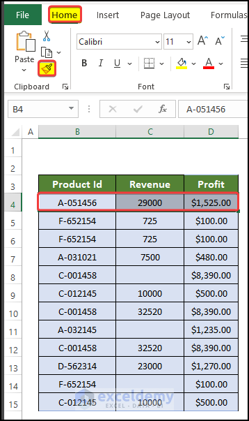
3. Then select only the B4:D4, and copy the formatting style of this cell.
4. Paste the formatting style all over the range of B4:D15.
And now you can see that the rows now highlighted if there is any blank cell in the entire row.
Thanks a lot for your question. Here, if all of the cells on a single row are blank in your dataset, they will be highlighted if you follow this tutorial. If you have any further issues, feel free to inform us again.
Thanks for your question James, I am not quite sure in which step you get the first error. You can better opt for an alternative approach.
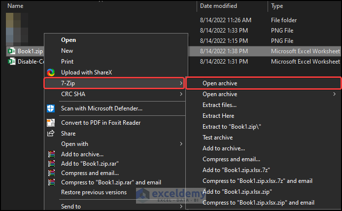
1. The procedure above should be followed until the first extension change. After the extension is changed to .zip, use the 7-zip application to open the archive, not to extract the zip.
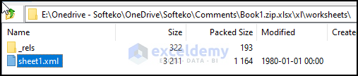
2. Then inside the archive, go to xl>worksheet. and double click on the sheet1.xml to edit the text as mentioned in the post.
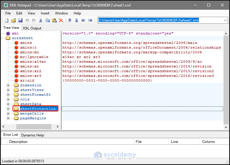
3. you can use a regular notepad application for opening the XML file. Or you can also opt for an XML notepad(https://microsoft.github.io/XmlNotepad/##_top) instead of a regular notepad. using the XML notepad, you can delete the protection part directly as a folder, as shown in the image.
4. After deleting the protection part, save the XML file.
5. And then change the extension part back to xls.
6. You will see that the Excel file is now unprotected.
Last but not the least, try to use Microsoft Office 365 instead of regular version of Excel.That way you will always be ensured with the latest updates.