How to Use Excel VBA to Filter a Pivot Table (5 Examples)

Method 1 – Filter a Pivot Table Based on Single Criteria Using VBA

STEPS:

• To create a pivot table, a sample code is given below.
• The user must first open the VBA editor following the Developer tab >> Visual Basic.
• In the “Microsoft Visual Basic for Applications” window, click Insert >> Module.
• After opening the editor, paste the code below into the editor. Then press the Run command.

Sub CreatePivotTableWithFilter()
Dim dataRange As Range
Set dataRange = ActiveSheet.Range("B4:F19")
Dim pivotDestination As Range
Set pivotDestination = ActiveSheet.Range("B22")
Dim pivotTable As pivotTable
Set pivotTable = ActiveSheet.PivotTables.Add(PivotCache:= _
ActiveWorkbook.PivotCaches.Create(SourceType:=xlDatabase, SourceData:= _
dataRange), TableDestination:=pivotDestination, TableName:="PivotTable4")
With pivotTable
.PivotFields("Region").Orientation = xlRowField
.AddDataField .PivotFields("Sales"), "Total Sales", xlSum
.AddDataField .PivotFields("Quantity"), "Total Quantity", xlSum
End With
End Sub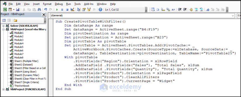

• After pressing Run, we will see that the worksheet has a pivot table with field properties set in the code.
• We can modify this code and add a filter to the pivot table.
  • Enter the following code into the VBA editor:

Sub CreatePivotTableWithFilter()
Dim dataRange As Range
Set dataRange = ActiveSheet.Range("B4:F19")
Dim pivotDestination As Range
Set pivotDestination = ActiveSheet.Range("B23")
Dim pivotTable As pivotTable
Set pivotTable = ActiveSheet.PivotTables.Add(PivotCache:= _
ActiveWorkbook.PivotCaches.Create(SourceType:=xlDatabase, SourceData:= _
dataRange), TableDestination:=pivotDestination, TableName:="PivotTable4")
With pivotTable
.PivotFields("Region").Orientation = xlRowField
.AddDataField .PivotFields("Sales"), "Total Sales", xlSum
.AddDataField .PivotFields("Quantity"), "Total Quantity", xlSum
.PivotFields("Product").Orientation = xlPageField
.PivotFields("Product").ClearAllFilters
.PivotFields("Product").CurrentPage = "Widget"
End With
End Sub

• We can see that the pivot table has a Filter on top of the pivot table.
• Switching the values on the pivot table will change the values in the pivot table.

Read More: Excel VBA to Filter Pivot Table Based on Cell Value

Method 2 – Filter a Pivot Table Based on Multiple Criteria Using VBA

In the previous method, we saw how to create a Pivot table with a filter. Now, in this method, we will discuss how we can create a pivot table that will have a filter with multiple-choice options. Meaning we can filter table values based on two or more separate criteria at the same time.

Sub Multiple_FILTER()
Dim pt As pivotTable
Dim PF_PRODUCT As PivotField
Set pt = ThisWorkbook.Worksheets("Data").PivotTables("Dataset")
Set PF_PRODUCT = ActiveSheet.PivotTables("Dataset").PivotFields("Product")
PF_PRODUCT.ClearAllFilters
PF_PRODUCT.EnableMultiplePageItems = True
PF_PRODUCT.PivotItems("Widget").Visible = False
PF_PRODUCT.PivotItems("Remote").Visible = False
Set PF_PRODUCT = Nothing
Set pt = Nothing
End Sub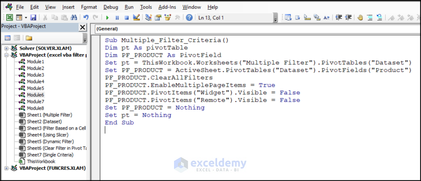

Read More: Excel VBA to Filter Pivot Table Based on Multiple Cell Values

Method 3 – Filter Based on Cell Value

STEPS:

• Create a Pivot table with the Region in the row field and the Quantity and the Sales in the values field.
• Filter the values according to the Product name.
• Open the VBA editor following the Developer tab >> Visual Basic.
• In the “Microsoft Visual Basic for Applications” window, click Insert >> Module.
• Paste the code below to the editor. Then press the Run command.

Sub Pivot_Table_Filter_Based_on_Cell_Value()
Dim dataRange As range
Set dataRange = ActiveSheet.range("B4:F19")
Dim pivotDestination As range
Set pivotDestination = ActiveSheet.range("B23")
Dim pivotTable As pivotTable
Set pivotTable = ActiveSheet.PivotTables.Add(PivotCache:= _
ActiveWorkbook.PivotCaches.Create(SourceType:=xlDatabase, SourceData:= _
dataRange), TableDestination:=pivotDestination, TableName:="PivotTable25")
With pivotTable
.PivotFields("Region").Orientation = xlRowField
.AddDataField .PivotFields("Sales"), "Total Sales", xlSum
.AddDataField .PivotFields("Quantity"), "Total Quantity", xlSum
.PivotFields("Product").Orientation = xlPageField
.PivotFields("Product").ClearAllFilters
.PivotFields("Product").CurrentPage = ActiveSheet.range("E22").Value
End With
End Sub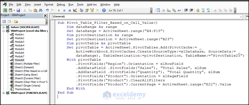

• After pressing the Run command, we can see that the PivotTable has been created with the mentioned fields and a filter button at the top.
• The interesting part is that the filter button criteria depend on the cell value of the cell. The Filter button will choose the value to apply a filter on the pivot table, the same as the value in cell E22.
• If we change the value in cell E22 to something else, the filter criteria also change, and the value in the pivot table is updated accordingly.

Method 4 – Use Slicers to Filter Pivot Tables

STEPS:

• Have a pivot table ready to apply the slicer.
• The pivot table from the dataset is created and given below.

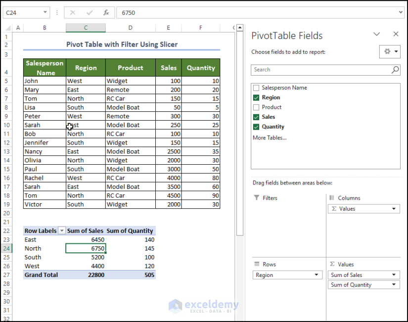
• We have that Region in the Row field and the Sum of Sales and Quantity in the values fields.
• Add the slicer to the worksheet.
  • Oen the VBA code editor from the Developer tab, as mentioned before.
  • In the code editor, enter the following code:

Sub AddSlicerToPivotTable()
Dim sl As slicer
Dim pt As pivotTable
Dim slic_cache As SlicerCache
Set pt = ThisWorkbook.Worksheets("Using Slicer").PivotTables("PivotTable2")
Set slic_cache = ThisWorkbook.SlicerCaches.Add2(pt, "Product", "ProductCache", XlSlicerCacheType.xlSlicer)
Set sl = sli_cache.Slicers.Add(slicerdestination:=Worksheets("Using Slicer"), Name:="slicer2")
End Sub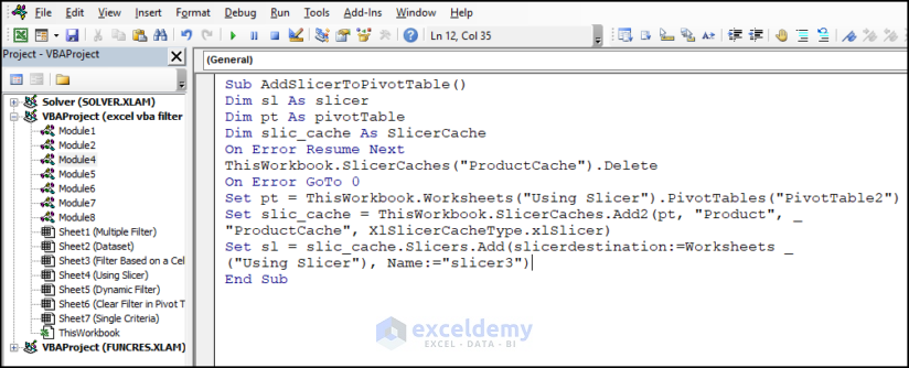

• After entering this code, we can see a slicer in the worksheet. You can filter the value in the pivot table based on the value you choose for the slicer.
• As you look through the values in the Slicer, the values in the Pivot table also change accordingly.

Method 5 – Creating Dynamic Filters with VBA

STEPS:

• We will present code that adds a pivot table and filter to the worksheet. The pivot table filter will be dynamic and depend on cell value E22.
• Right-click on the sheet name panel and click on the View Code.
• In the code editor, paste the code given below.
• Inside the module, paste the code given below:

Private Sub Worksheet_Change(ByVal Target As range)
If Target.Address = "$E$22" Then
Dim dataRange As range
Set dataRange = Me.range("B4:F19")
Dim pivotDestination As range
Set pivotDestination = Me.range("B23")
Dim pivotTable As pivotTable
Dim ws As Worksheet
Dim pt As pivotTable
On Error Resume Next
Set ws = Worksheets("Dynamic Filter")
Set pt = ws.PivotTables("PivotTable16")
pt.TableRange2.Clear
Set pivotTable = Me.PivotTables.Add(PivotCache:= _
ActiveWorkbook.PivotCaches.Create(SourceType:=xlDatabase, SourceData:= _
dataRange), TableDestination:=pivotDestination, TableName:="PivotTable16")
With pivotTable
.PivotFields("Region").Orientation = xlRowField
.AddDataField .PivotFields("Sales"), "Total Sales", xlSum
.AddDataField .PivotFields("Quantity"), "Total Quantity", xlSum
.PivotFields("Product").Orientation = xlPageField
.PivotFields("Product").ClearAllFilters
.PivotFields("Product").CurrentPage = Me.range("E22").Value
End With
End If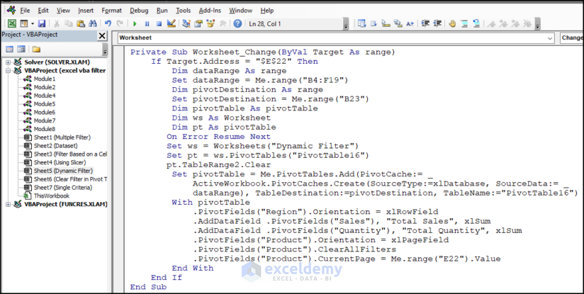

• As this code is a Private Sub, you do not need to run the code manually from the view tab.
• When you change the value of cell E22, the code executes automatically and shows the pivot table in the worksheet.
• The table will also filter the data based on the cell value in cell E22.

Clear Filters from the Pivot Table Using Excel VBA

STEPS:

• Have a pivot table in the worksheet. We have a pivot table already in the worksheet named, and the filter is applied to the Product field.
• The filter is now applied for Model Boat and Widget. We need to remove this filter from this pivot table.

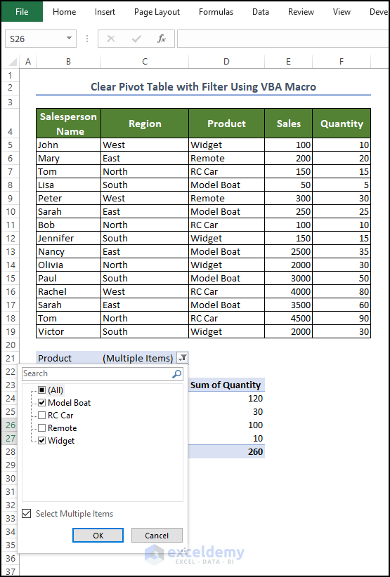
Sub Clear_Filter()
ActiveSheet.PivotTables("PivotTable3").PivotFields("Product").ClearAllFilters
End Sub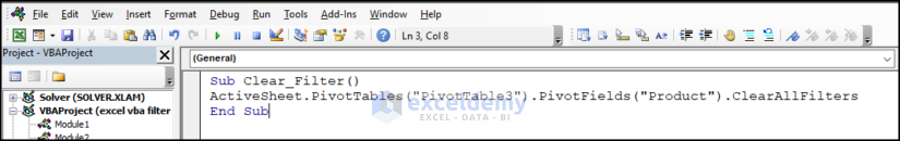

• We will see that the PivotTable3 is now free from any filter and now shows all the data points in the dataset.

Things to Remember

Pivot Table Structure: Filters are applied to the pivot table, not just specific rows or columns. So, when you apply a filter, it affects the visibility of data across the entire table.

Filter Types: Excel provides various types of filters in pivot tables, including label filters, value filters, and manual filters. Each type allows you to filter data based on different criteria.

Field Selection: Choose the correct field to apply the filter. Pivot tables have row fields, column fields, report filter fields, and value fields. Ensure you select the appropriate field to filter the data you want.

Filtering Options: Depending on the type of data in the field, you can use different filtering options. For example, text fields offer options like contains, begins with, ends with, etc., while number fields provide options like equals, greater than, less than, etc.

Multiple Filters: You can apply multiple filters to a pivot table. Each filter narrows down the data further, helping you focus on specific subsets of information.

Updating Filters: If the underlying data in your pivot table changes, you might need to update the filters to reflect the latest information. Right-click on the pivot table and select “Refresh” to update the filters and the entire pivot table.

Clearing Filters: To remove filters and display the entire dataset, right-click on the pivot table, select “Clear Filter,” and choose the appropriate option to clear the filters.

Grouping Data: In addition to filters, you can also group data in a pivot table. Grouping allows you to combine and summarize data based on specific criteria, such as date ranges or custom categories.

Saving Filters: Excel does not save filters within the pivot table. If you save the workbook and reopen it later, the filters will be cleared. If you want to preserve specific filter settings, you can create a copy of the filtered pivot table or save the filtered data in a separate worksheet.

Filter Interactions: Filters in a pivot table can interact with each other. When you apply multiple filters, they can affect each other’s results. Be mindful of the filter order and how they impact the data visibility.

Download the Practice Workbook

Download the following workbook to practice.

Related Articles

• Excel VBA to Filter Pivot Table Based on List
• Excel VBA Pivot Table to Filter Between Two Dates