Excel Pivot Table Date Filter Not Working (2 Possible Solutions)

Reason 1 – All Cells of a Column Are Not in Date Format

One of the most common reasons the pivot table date filter might not work is that all the data are not in the proper date format. Although a cell containing a date might look like a date-formatted one at a glance, it can actually be in text format.

Reason 2 – The AutoFilter Grouping Date Option Is Not Enabled

Another big reason for the pivot table date filter not working is that the group dates option in the auto filter menu is disabled. This option status is found in the Advanced tab of Excel Settings.

Pivot Table Date Filter Not Working Issue: 2 Solutions

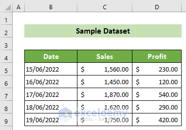
We have a dataset of five days’ worth of dates, sales, and profits.

We have created a pivot table according to this dataset.

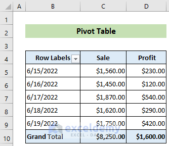
When we tried to apply the date filter in the pivot table, it did not work properly.

Fix 1 – Ensure the Date Format for the Entire Column

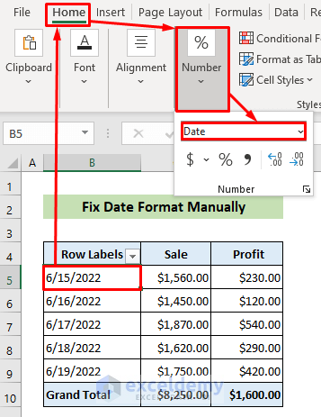
Case 1.1 – Fix the Format Manually

Steps:

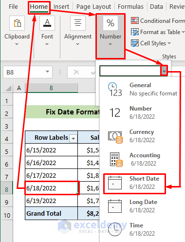
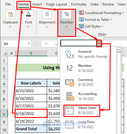
• Click on the B5 cell. Go to the Home tab and, in the Number group, note the format inside the Number Format text box. The B5 cell’s value is in the Date format.

• Repeat this process for all the Date column cells. At the B8 cell, you can see that the value is in the Text format.

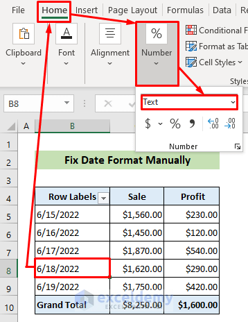
• With the cell selected, click on the drop-down arrow inside the Number Format text box and choose the Short Date option from the listed options.

Case 1.2 – Using the ISTEXT Function

Steps:

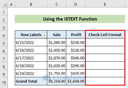
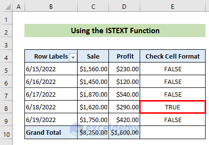
• Create a new column next to the pivot table named Check Cell Format.

• Select the E5 cell and insert the following formula.

• Press the Enter button.

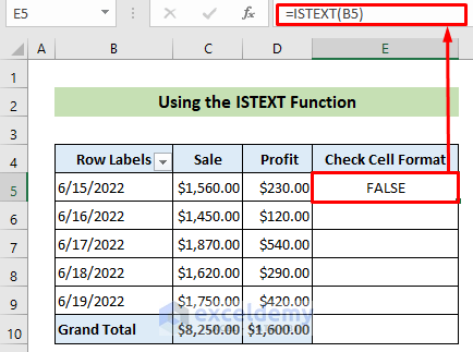
• You can see that FALSE is written in the E5 cell because the B5 cell has a date format value, not a text value.
• Place your cursor on the bottom-right corner of the E5 cell.
• The fill handle (plus icon) will appear. Drag the fill handle down to the E9 cell.

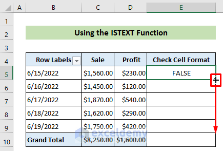
• The E8 cell returns the TRUE value. And you can find that the B8 cell has the text format value.

• Select the B8 cell, click on the drop-down arrow in the Number Format text box, and select the Short Date option.

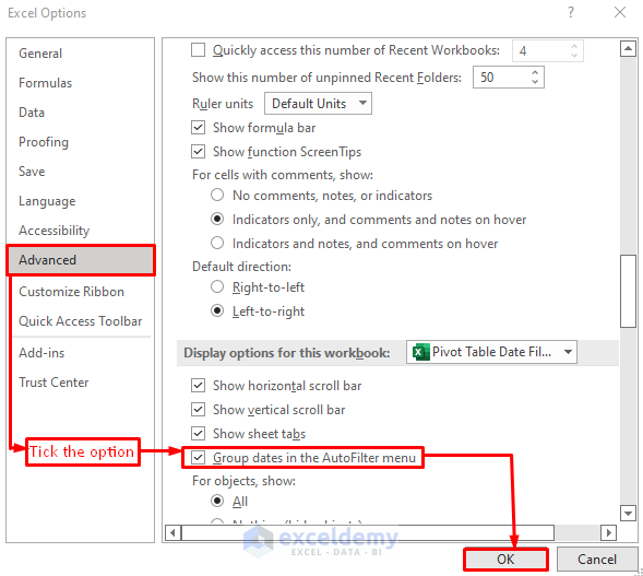
Fix 2 – Enable the AutoFilter for Grouping Dates

Steps:

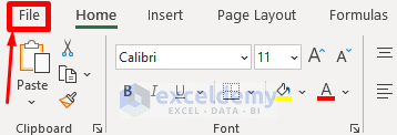
• Go to the File tab.

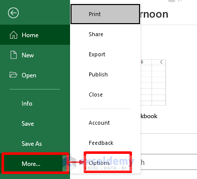
• Select Options (it could be under More at the bottom).

• The Excel Options dialog box will appear. Go to the Advanced tab.
• Check the option Group dates in the AutoFilter menu.
• Click on the OK button.

Download the Practice Workbook

Related Articles

• How to Create a Timeline in Excel to Filter Pivot Table
• How to Use Pivot Table to Filter Date Range in Excel