This is an overview:
Solution 1 – Replacing Missing or Distorted Date Values to Group Dates in a Pivot Table
Step 1:
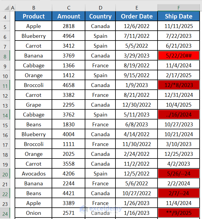
- There are error date values in the image below:
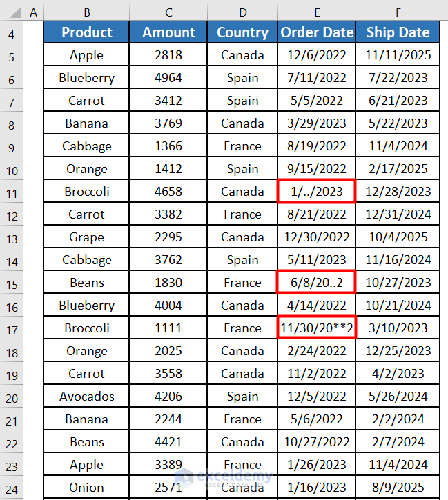
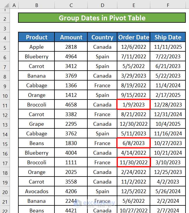
- 3 error dates were corrected.
Step 2:
- To group dates, create a pivot table: drag the cells as shown below:
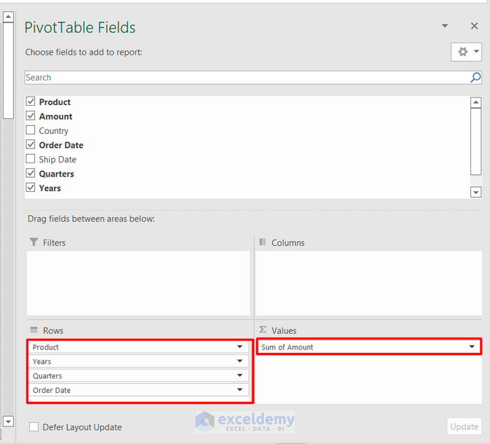
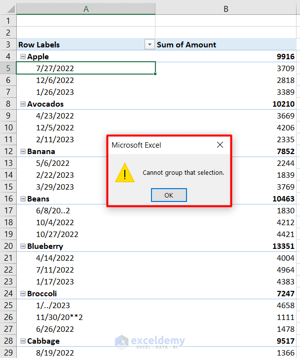
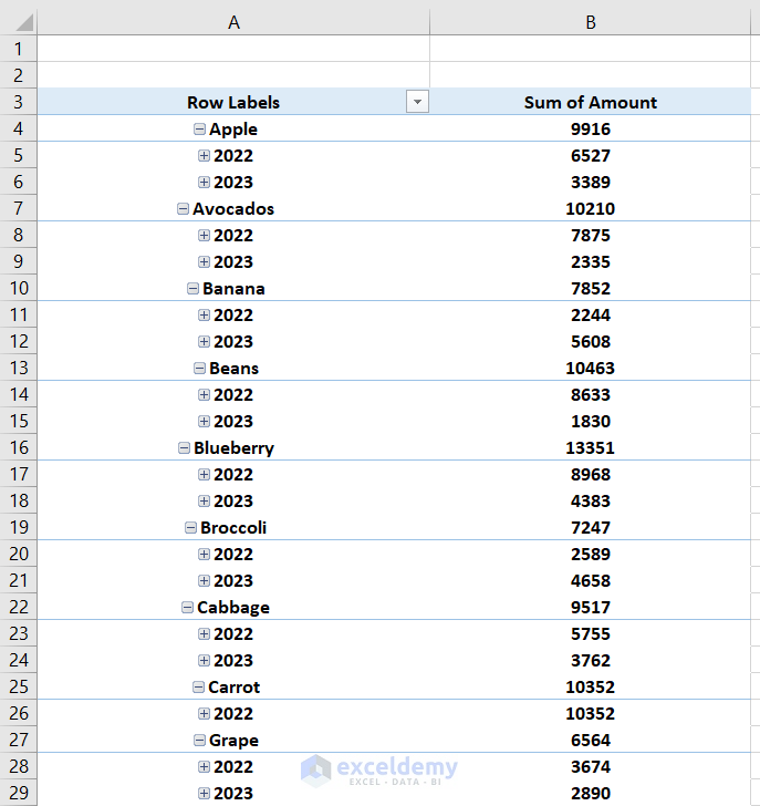
This is the pivot table:
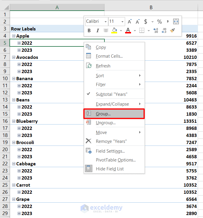
Step 3:
- Select any cell containing a year.
- Right-click it.
- Click Group.
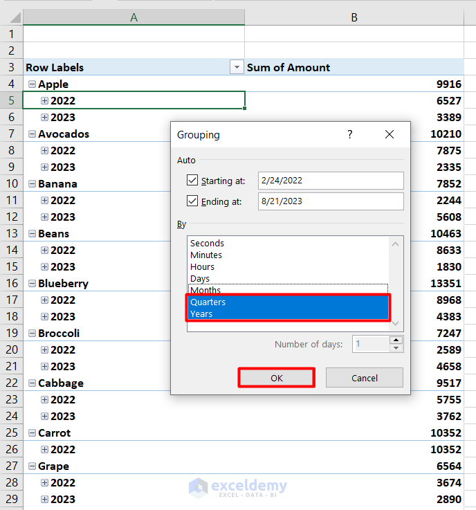
- In Grouping, select how to group data. Here, Quarters and Years.
- Click OK.
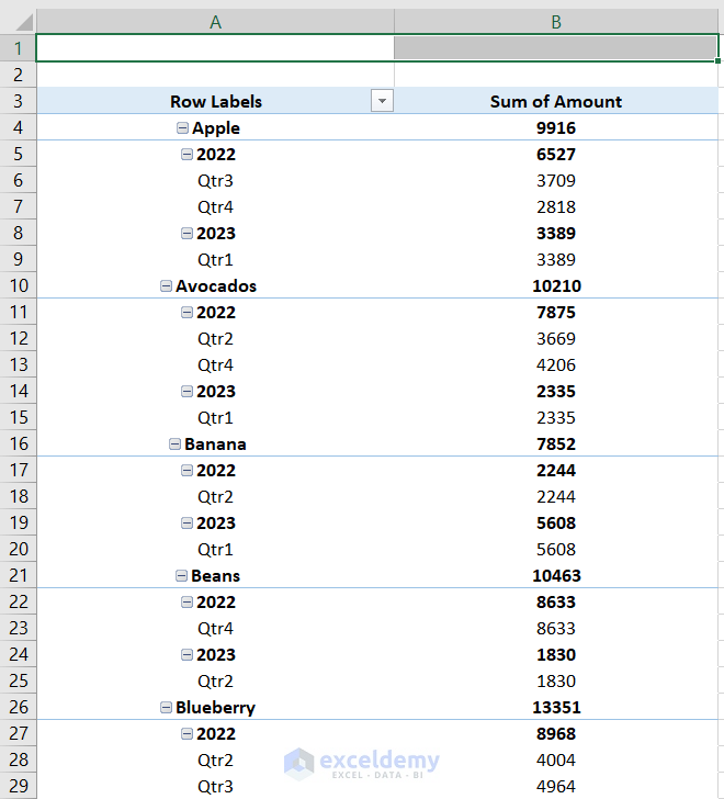
This is the output.
Read More: [Fixed] Excel Pivot Table Not Grouping Dates by Month
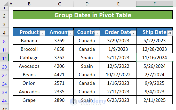
Solution 2 – Filtering to Find Distorted Date Values and Group Dates in Pivot Tables
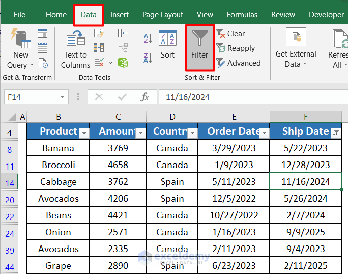
Step 1:
- Select all the cells in the data range.
- Click Filter in Data.
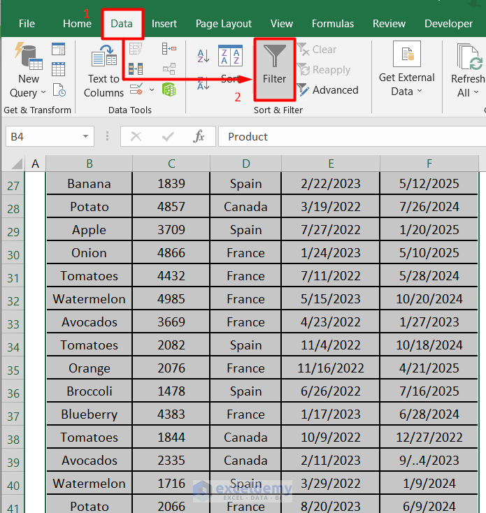
- Click the small downward arrow on the right side of Ship Date: The filter drop-down menu has grouped all date values in this column by Year, and Date. Text and error date values are at the bottom of the list.
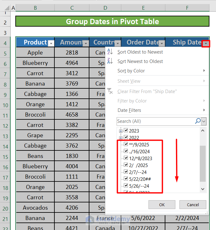
Step 2:
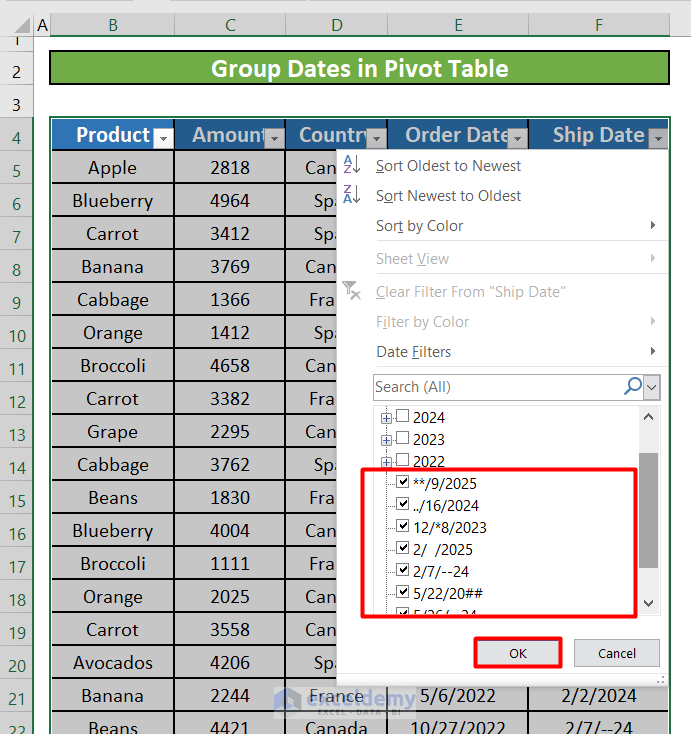
- To filter the Text and ERROR values, uncheck all the date items or uncheck Select All.
- Select the text and error items.
- Click OK.
The column will be filtered and display the text and error values.
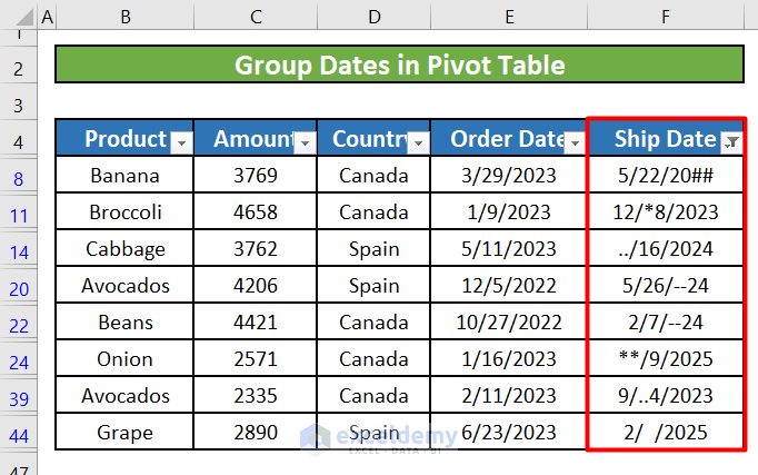
Step 3:
Correct the filtered dates with errors:
- Click Filter again.
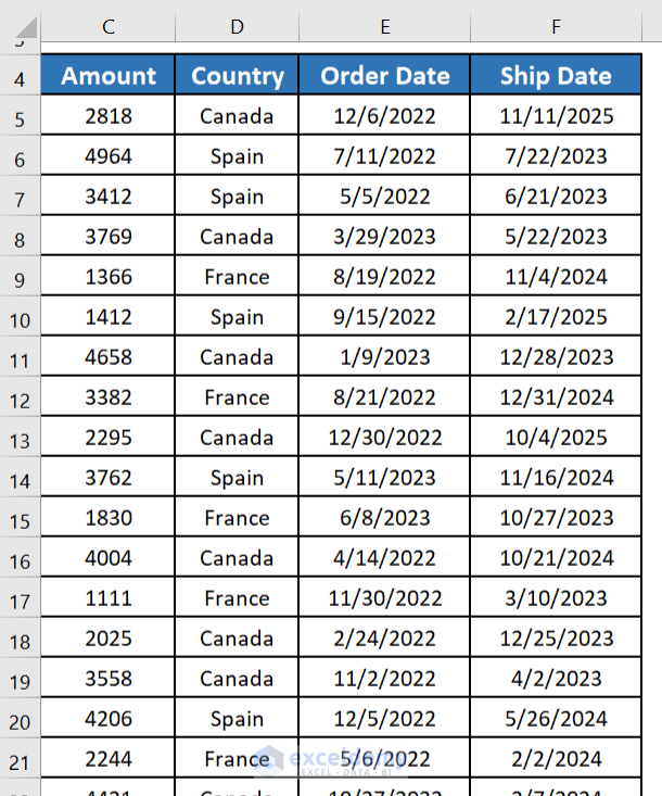
The data range will be displayed with corrected dates.
- Group the dates.
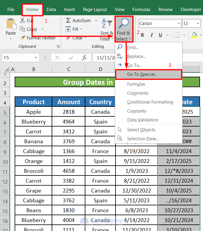
Solution 3 – Finding Error Date Values Using the GoTo Special Menu to Group Dates in the Pivot Table
Steps:
- Select the entire column in the date field. You can press CTRL+SPACE.
- Go to Find & Select in the Home tab.
- Select Go To Special.
- Select Constants.
- Uncheck Numbers.
- Click OK.
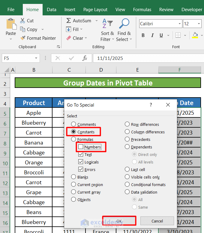
Cells containing text or error values will be selected.
- You can highlight these cells to fix the values. Here, in Red.
Solution 4 – Finding Error Date Values using VBA
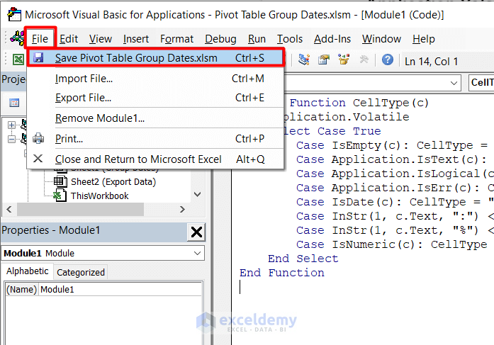
- Click ALT+F11 to open Visual Basic You can also open it in the Developer tab.
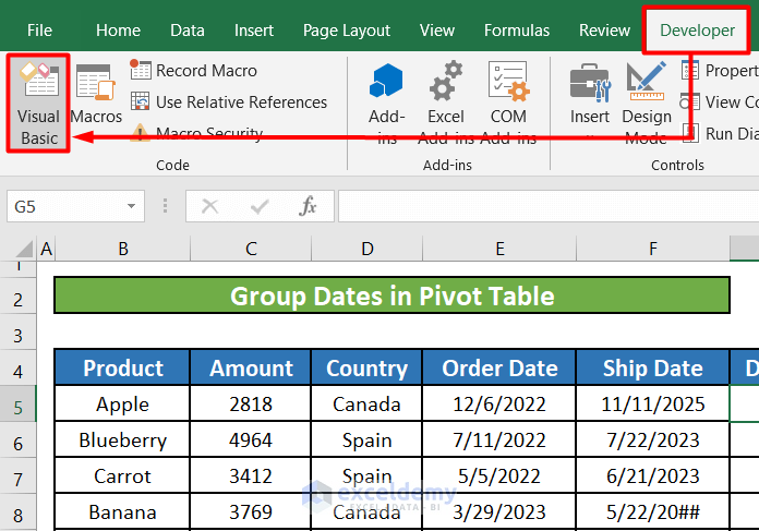
- Click Insert and select Module.
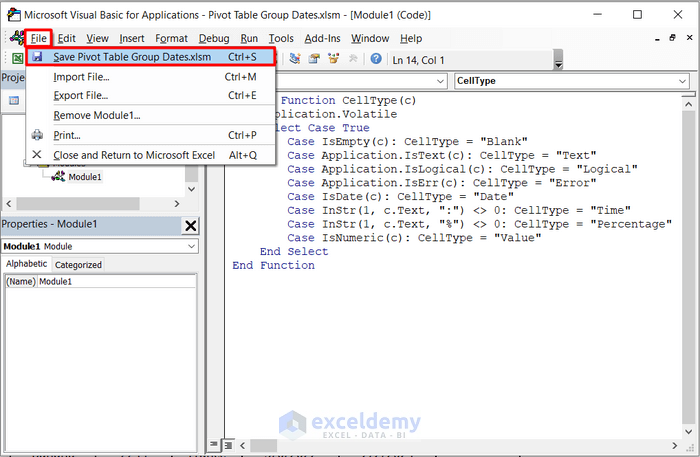
- Use the following code:
Public Function CellType(c)
    Application.Volatile
    Select Case True
        Case IsEmpty(c): CellType = "Blank"
        Case Application.IsText(c): CellType = "Text"
        Case Application.IsLogical(c): CellType = "Logical"
        Case Application.IsErr(c): CellType = "Error"
        Case IsDate(c): CellType = "Date"
        Case InStr(1, c.Text, ":") <> 0: CellType = "Time"
        Case InStr(1, c.Text, "%") <> 0: CellType = "Percentage"
        Case IsNumeric(c): CellType = "Value"
    End Select
End Function- Click the File tab and save the Excel file.
- Go back to the source worksheet and enter the following function in G5:
=CellType(F5)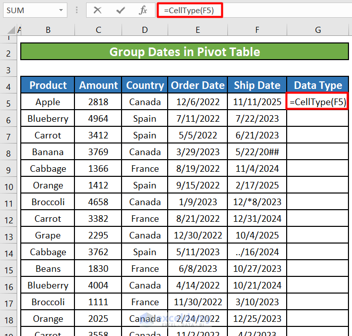
- Press ENTER.
You will see the data type used in F5.
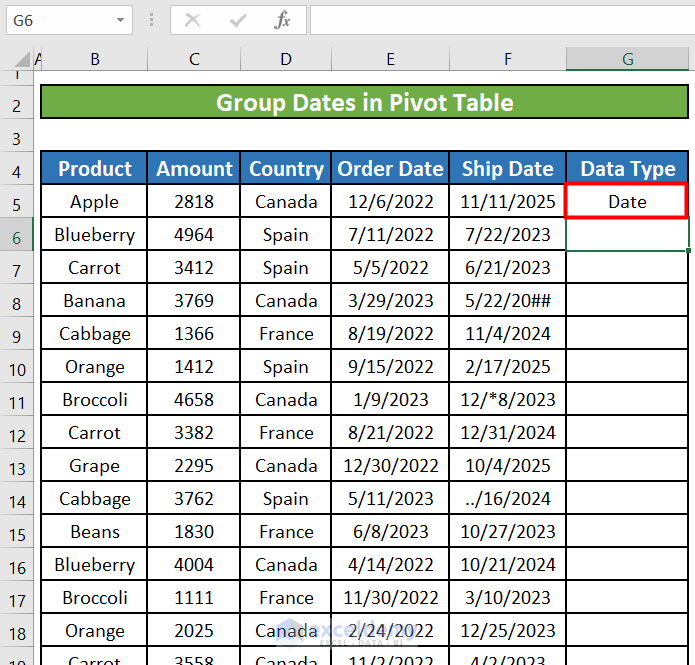
- Drag down the Fill Handle to see the result in the rest of the cells.
There is Text for dates with error values.
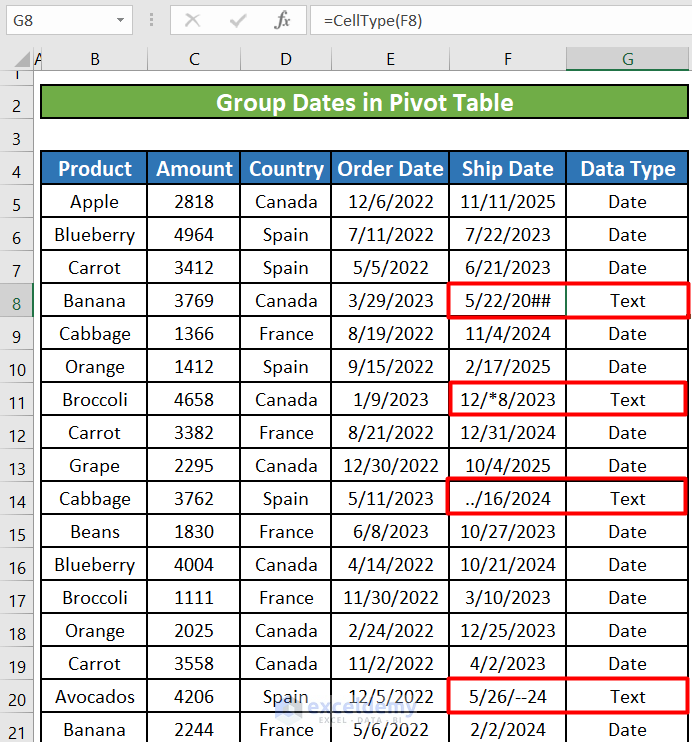
- Highlight the cells with Text to correct them.
Things to Remember
- You can also use the VBA CellType function to determine the type of data in a cell.
- Select New Worksheet when you are creating a pivot table.
Download Practice Workbook
Download this practice book.
Related Articles
- How to Group by Week in Excel Pivot Table
- How to Group by Month in Excel Pivot Table
- How to Group by Year in Excel Pivot Table
- How to Group by Week and Month in Excel Pivot Table
- How to Group by Month and Year in Excel Pivot Table
<< Go Back to Group Dates in Pivot Table | Group Pivot Table | Pivot Table in Excel | Learn Excel
Get FREE Advanced Excel Exercises with Solutions!
