How to Group by Month in Excel Pivot Table?

Method 1 – Group Pivot Table Manually by Month

STEPS:

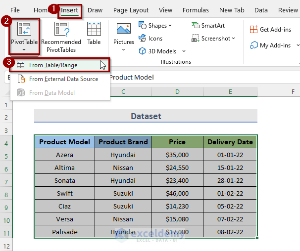
• Select the whole dataset and go to the Insert tab on the ribbon.
• From the Insert tab, go to the PivotTable drop-down menu and select From Table/ Range.

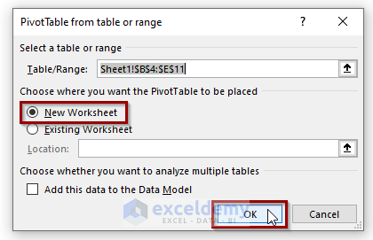
• This will open the PivotTable from table or range dialog box. There we can see that the Table/Range is already selected.
• From Choose where you want the PivotTable to be placed option, we can choose the location where we want the pivot table. We want to place our table on a new worksheet. We chose New Worksheet.
• Click OK.

• The pivot table is created in a new sheet.

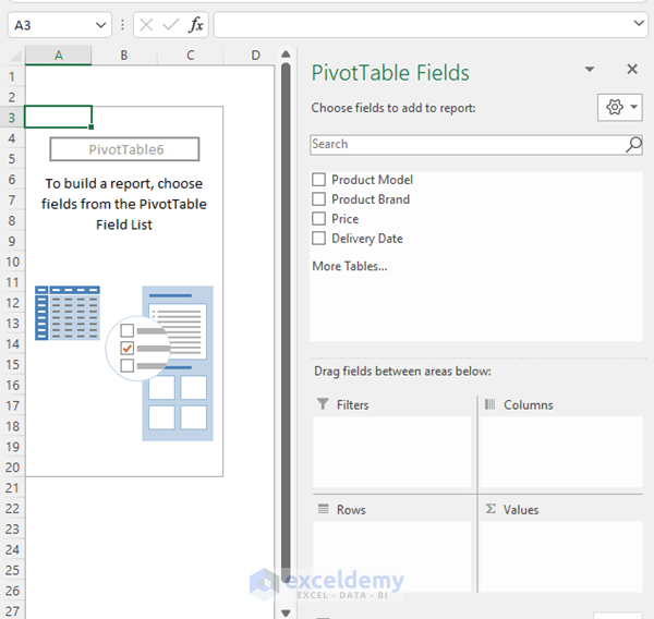
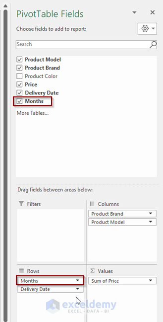
• In the PivotTable Fields, we will customize the table. We put the product brand and model in the Columns area and the price in the Values We will put the delivery date in the Rows area.

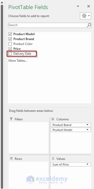
• Dragging the delivery date to the Rows area will create the month automatically. In the image below, there is another field which is Months.

• The pivot table is grouped by January and February.

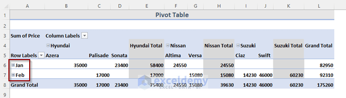
• We can extend the data by clicking on the plus (+) sign.

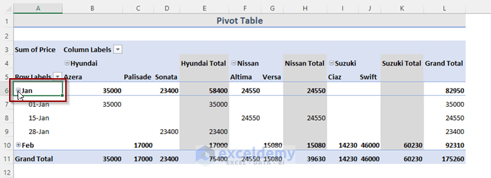
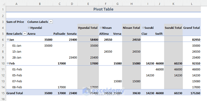
• The dates can also be viewed.

Read More: How to Group by Week in Excel Pivot Table

Method 2 – Automatically Group Pivot Table by Month

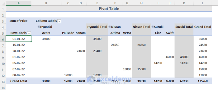
Assume that, we want to group the data by month in this pivot table.

STEPS:

• Select any cell in the Row Labels, where the delivery date is located.

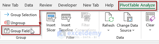
• Go to the PivotTable Analyze tab on the ribbon.
• Select the Group Field in the group section.

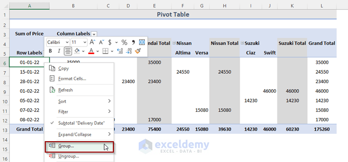
• Or right-click on the mouse and select the Group.

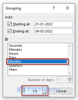
• The Grouping dialog box will appear. In this window, we can see that the starting date and ending dates are automatically set.
• Select the Months and click on OK.

• This will group the pivot table by months.

Read More: How to Group by Year in Excel Pivot Table

How to Ungroup a Pivot Table in Excel?

STEPS:

• Select the grouped data on the pivot table.
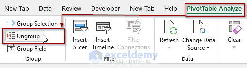
• Go to the PivotTable Analyze tab > Ungroup.

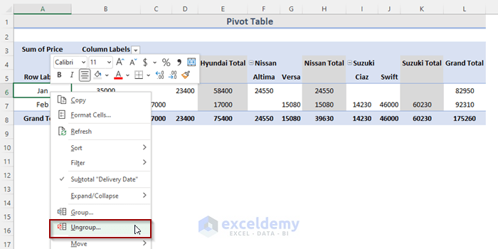
• Or, right-click on the grouped data on the pivot table and select Ungroup.

Read More: How to Group by Week and Month in Excel Pivot Table

Download Practice Workbook

Related Articles

• How to Group by Month and Year in Excel Pivot Table
• [Fix] Cannot Group Dates in Pivot Table
• [Fixed] Excel Pivot Table Not Grouping Dates by Month

<< Go Back to Group Dates in Pivot Table | Group Pivot Table | Pivot Table in Excel | Learn Excel