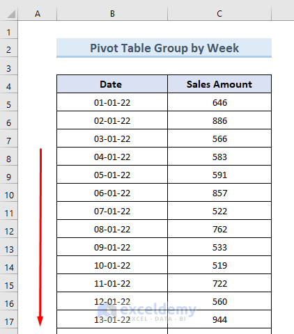
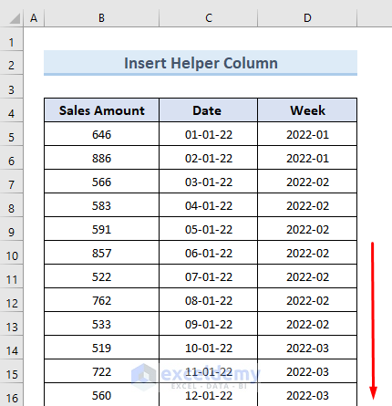
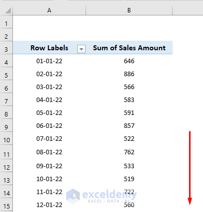
The following dataset showcases sales amounts in January.
Method 1 – Setting 7 Days As a Week to Group a Pivot Table by Week
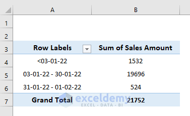
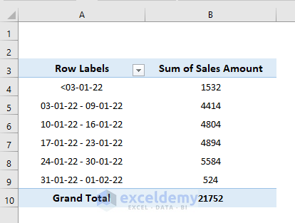
This is the pivot table of the previous dataset. The group selection method will be used, counting the number of days as 7.
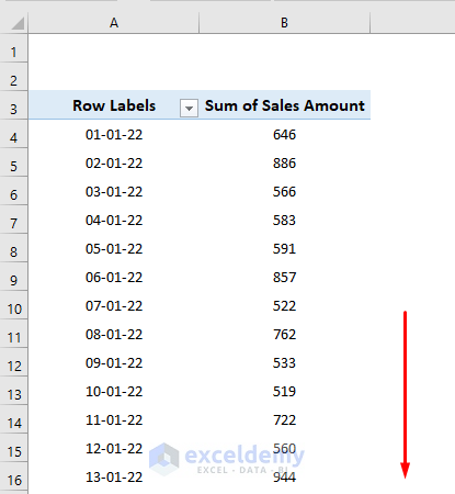
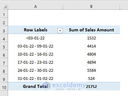
The week count will start from January, 3.

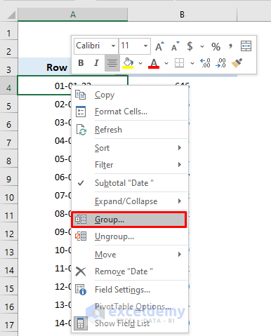
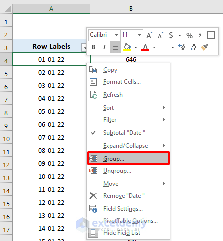
- Select any date in the pivot table.
- Right-click.
- Select Group.
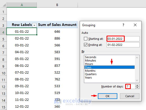
- In the dialog box, enter starting date 3-01-2022.
- Select Days.
- Enter 7 in Number of Days .
- Click OK.
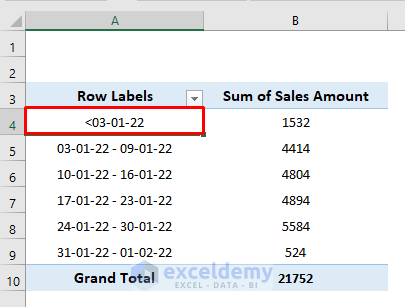
The pivot table is grouped by week. 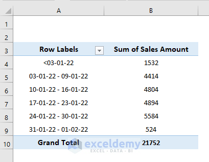
Read More: How to Group by Month in Excel Pivot Table
Method 2 – Using 4-Week Periods to Group Data in a Pivot Table
Group data of whole months:
- Select any date in the pivot table.
- Right-click.
- Select Group.
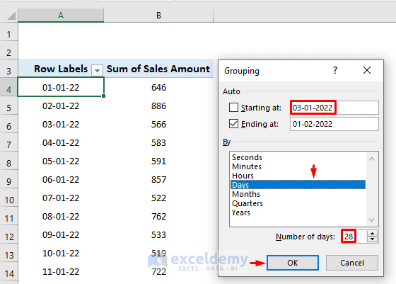
- In the dialog box, enter starting date 3-01-2022.
- Select group by Days.
- Enter 28 in Number of days.
- Click OK.
The pivot table is filtered by a 4-week period.
Read More: How to Group by Year in Excel Pivot Table
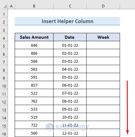
Method 3 – Inserting a Helper Column to Group a Pivot Table by Week
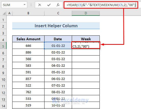
A new column (Week) was inserted in the previous dataset.

- Select D5. Use the following formula:
=YEAR(C5)&"-"&TEXT(WEEKNUM(C5,2),"00")- Press Enter.
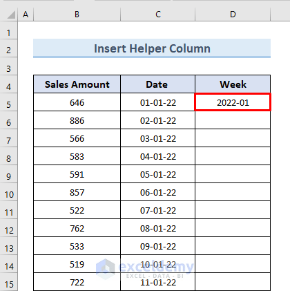
The number of weeks is displayed in C5.
Formula Breakdown
- WEEKNUM(C5,2),”00″: returns the number of weeks of the date value in C5.
- TEXT(WEEKNUM(C5,2),”00″: Extracts the text value of the week.
- YEAR(C5)&”-“&TEXT(WEEKNUM(C5,2),”00”: Returns the value of week with Year.
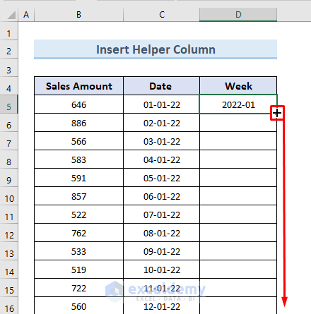
- Drag down the Fill Handle or double-click the (+) sign to get the number of weeks for all dates.
This is the output.
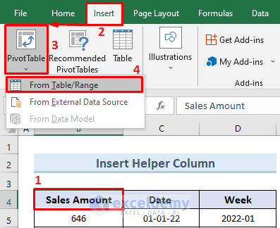
- To create a pivot table, select any cell from the data range. Here, D4.
- Go to the Insert tab and select Pivot Table.
- Choose From Table/Range.
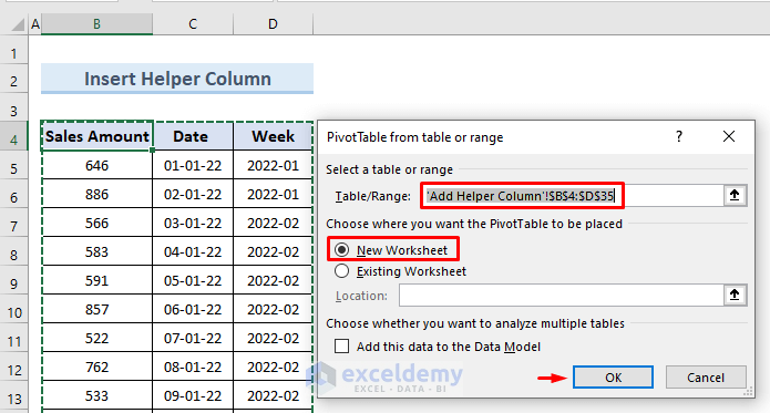
- In the dialog box, check New Worksheet and click OK.
A new window will be displayed.
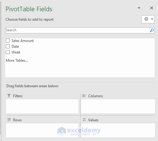
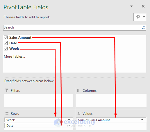
- Drag Week and drop it in the first place of the section Rows.
- Drag Date and drop it in the second place of the section Rows.
- Drag Sales Amount and drop it in the ⅀ Values section.
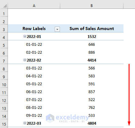
A pivot table grouped by week is displayed.
Read More: How to Group by Week and Month in Excel Pivot Table
How to Ungroup Week Data in a Pivot Table?
1. Using the Right-Click Option
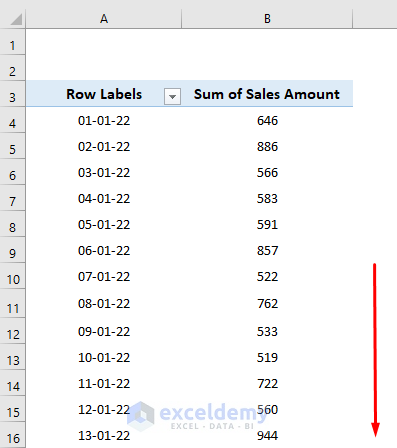
The following dataset is grouped by week.
- Select any cell in the pivot table.
- Right-click.
- Select Ungroup.
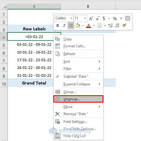
Data in the pivot table will be ungrouped.
2. With the PivotTable Analyze Tab
- Select any cell from the data range.
- Go to the PivotTable Analyze tab.
- In Group, select Ungroup.
The pivot table is ungrouped.
Things to Remember to Troubleshoot Errors
To avoid errors:
- Create a group with a minimum of two.
- Make sure there are no blank cells.
- Do not enter a text value in a date or numeric field or vice versa.
Download Practice Workbook
You can download the practice workbook here.
Related Articles
- How to Group by Month and Year in Excel Pivot Table
- [Fix] Cannot Group Dates in Pivot Table
- [Fixed] Excel Pivot Table Not Grouping Dates by Month
<< Go Back to Group Dates in Pivot Table | Group Pivot Table | Pivot Table in Excel | Learn Excel
Get FREE Advanced Excel Exercises with Solutions!
