If you want to create Excel Pivot Table Group Dates by Month and Year, this article is for you. Here, we will walk you through 4 simple and easy methods to do the task effortlessly.
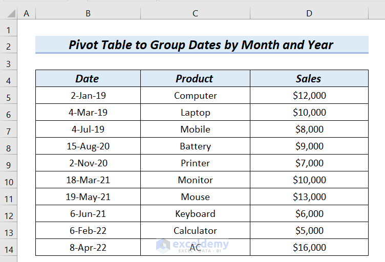
The following table has the Date, Product, and Sales columns. We want to create a Pivot Table to group dates by month and year for this table. To do so, we will go through 4 easy methods. All these methods are described step by step. In this article, we used Excel 365. You can use any available Excel version.
1. Using Group Option from Context Menu to Group Dates by Month and Year in Pivot Table
In this method, first, we will insert a Pivot Table. After that, we will use the Group option from the Context Menu to group Pivot Table by Month and Year. But before moving into that we will need to disable automatic grouping.
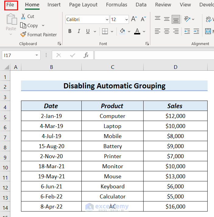
Step 1: Disabling Automatic Grouping
If you have Excel 2016 or any higher version of Excel, you will notice that the dates are grouped automatically when the dates are kept in a row or column of the Pivot Table. To avoid this automatic grouping, you have to follow the following steps.
- First, go to the File tab of your Excel sheet.
- After that, select Options.

An Excel Options dialog box will appear.
- Afterward, select Data >> mark or click on Disable automatic grouping of Date/Time columns in PivotTable.
- Then, click OK.

This will disable the automatic grouping. Now, we will start our article.
Step 2: Grouping Dates by Month and Year
- First, we will select the entire dataset >> go to the Insert tab.
- After that, select PivotTable >> select From Table/Range.

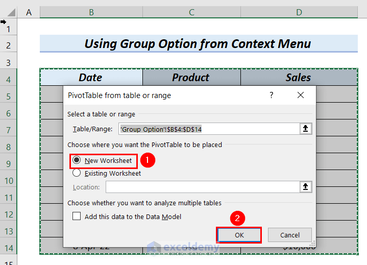
A PivotTable from table or range dialog box will appear.
- Then, we will select New Worksheet >> click OK.
Now, a new sheet will arrive for our Pivot Table. On the right side of the sheet, we will see PivotTable Fields.
- After that, we will drag the Date and Sales to the Rows and Values area respectively.
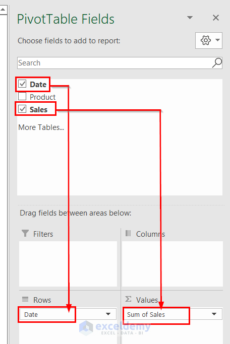
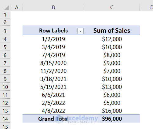
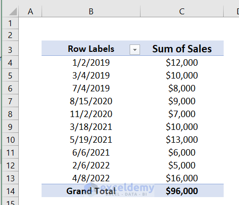
Now, we can see the PivotTable with the Row Labels, and Sum of Sales columns.
Next, we will group the dates by month and year in the Row Labels column.

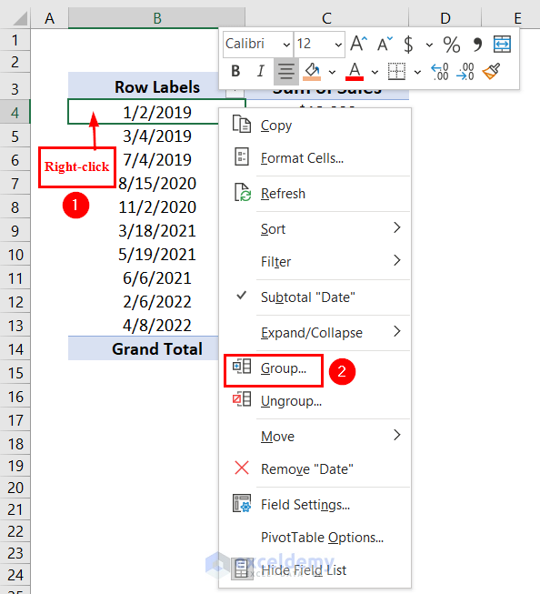
- Afterward, we will right-click on any of the cells of the Row Labels column.
- Here, we right-clicked on cell B4.
- Then, we will select the Group option from the Context Menu.
A Grouping dialog box will appear.
- After that, select the Month and Year.
- Then, click OK.

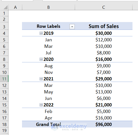
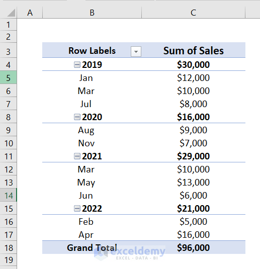
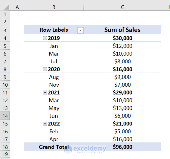
Finally, you will see grouped Dates by Month and Year in the Pivot Table.
Read More: How to Group by Week and Month in Excel Pivot Table
2. Using Group Selection Feature to Group Dates by Month and Year in Pivot Table
In this method, first, we will insert a PivotTable. After that, we will use the Group Selection feature from the PivotTable Analyze tab to group the pivot table by year and month.

Steps:
- First, we will insert a PivotTable by following the steps of Method-1.
- After that, we click on a date in the Row Labels column. Here, you can click on any of the cells of the Row Labels column.
- Then, we go to the PivotTable Analyze tab >> from Group >> select Group Selection.

A Grouping dialog box will appear.
- After that, select the Month and Year.
- Then, click OK.

Therefore, you will see grouped dates by Month and Year in the Pivot Table.
3. Applying Group Field Command
In this method, first, we will insert a PivotTable. After that, we will use the Group Field command from the PivotTable Analyze tab to group dates by Month and Year.

Steps:
- First, we will insert a PivotTable by following the steps of Method-1.
- After that, we click on a date in the Row Labels column. Here, you can click on any of the cells of the Row Labels column.
- Then, we go to the PivotTable Analyze tab >> from Group >> select Group Field.

A Grouping dialog box will appear.
- After that, select the Month and Year.
- Then, click OK.

As a result, you will see that all the dates are grouped by Month and Year in Excel Pivot Table.
4. Use PivotTable Fields to Group Dates By Month and Year
Here, we will add Year and Month columns to our dataset, therefore, there will be Year and Month fields in the PivotTable. As a result, when we will drag the Year and Month in the Row area of the PivotTable, it will group the date by Month and Year.
Steps:
- First, we will type the following formula in cell E5.
=YEAR(B5)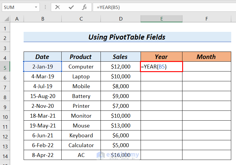
Formula Breakdown
- YEAR(B5) → The YEAR function returns a year corresponding to a Date.
- YEAR(2-Jan-19) → becomes
- Output: 2019
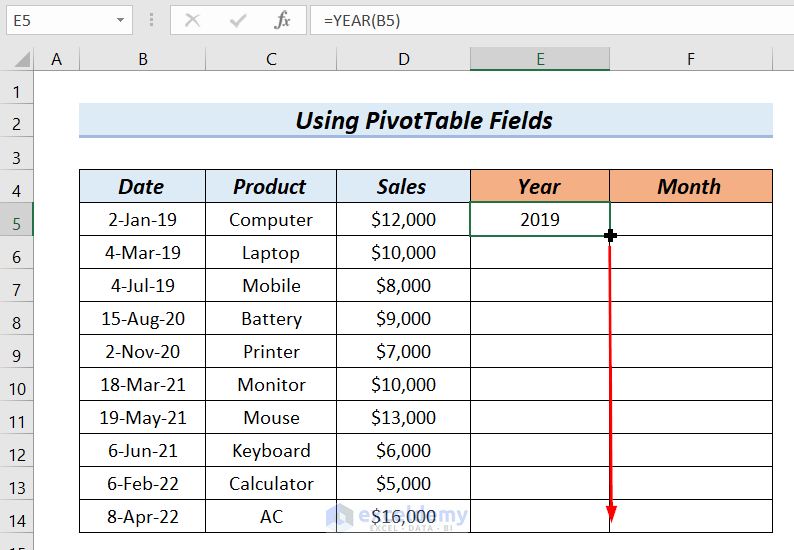
- After that, press ENTER. Then, you will see the result in cell E5.
- Afterward, we will drag down the formula with the Fill Handle tool.
- Afterward, we will write the following formula in cell F5.
=TEXT(B5,"mmmm")
Formula Breakdown
- TEXT(B5,”mmmm”) → The TEXT function changes the way a number appears by formatting it using format codes.
- B5 is the value to format.
- “mmmm” is the format code to apply.
- TEXT(2-Jan-19,”mmmm”) becomes
- Output: January
- After that, press ENTER. Then, you will see the result in cell E5.
- Afterward, we will drag down the formula with the Fill Handle tool.

Now, we will insert a PivotTable.
- First, we will select the Entire Dataset >> go to the Insert tab.
- After that, select PivotTable >> select From Table/Range.

A PivotTable from table or range dialog box will appear.
- Then, we will select New Worksheet >> click OK.

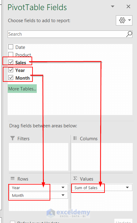
Now, a new sheet will arrive for our Pivot Table. On the right side of the sheet, we will see PivotTable Fields.
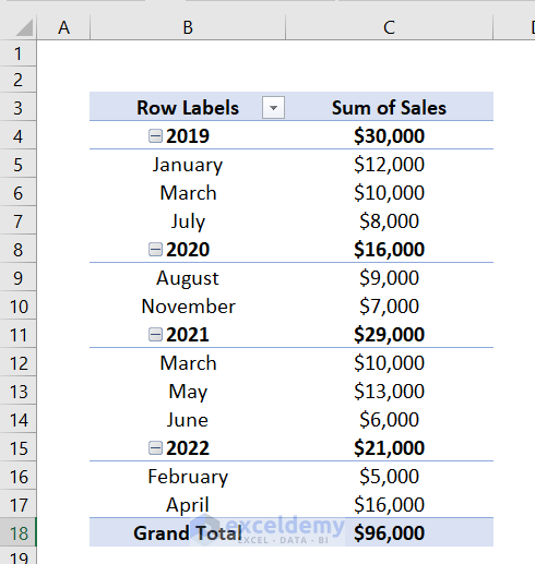
- After that, we will drag the Year and Month to the Rows area, and the Sales to the Values area.
Therefore, you will see that all the Dates are Grouped by Month and Year in Excel Pivot Table.
Download Practice Workbook
Conclusion
Here, we tried to show you 4 methods to use a pivot table to group dates by Month and Year in Excel. Thank you for reading this article, we hope this was helpful. If you have any queries or suggestions, please let us know in the comment section below. Please visit our website to explore more.
Related Articles
- How to Group by Week in Excel Pivot Table
- [Fix] Cannot Group Dates in Pivot Table
- [Fixed] Excel Pivot Table Not Grouping Dates by Month
<< Go Back to Group Dates in Pivot Table | Group Pivot Table | Pivot Table in Excel | Learn Excel
Get FREE Advanced Excel Exercises with Solutions!
