While working with Microsoft Excel, sometimes we need to Group data by Week and Month in Pivot Table. Grouping data by Week and Month in Excel Pivot Table is an easy task. This is a time-saving task also. Today, in this article, we’ll learn three quick and suitable steps to group by Week and Month in Excel Pivot Table effectively with appropriate illustrations.
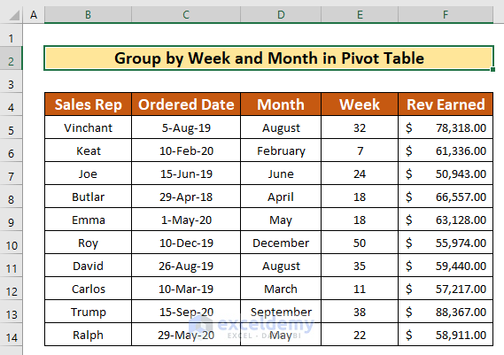
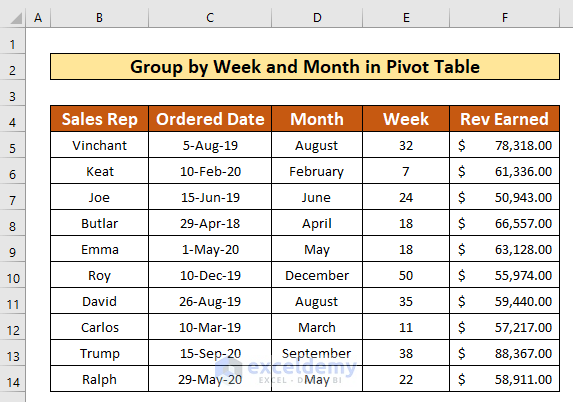
Let’s assume we have a large worksheet in Excel that contains information about several sales representatives of the Armani Group. The name of the sales representatives, the Ordered Date, and the Revenue Earned by the sales representatives are given in Columns B, C, and F respectively. From our dataset, we will group by week and month in the Pivot Table. To do that, firstly, we will calculate the Month and the Week from the Ordered Date using the TEXT and WEEKNUM functions. After that, we will group by week and month in the Pivot Table in Excel. Here’s an overview of the dataset for today’s task.
Step 1: Calculating the Number of Weeks and Months from Date in Excel
In this portion, we will calculate the Month and the Week using the TEXT and the WEEKNUM functions to group the pivot table by week and the month. This is an easy task and time-saving also. Let’s follow the instructions below to learn!
- First of all, select cell D5, and write down the below TEXT function to calculate the Month from the Ordered Date. The TEXT function is,
=TEXT(C5, "mmmm")- Where C5 is the value and mmmm is the format_text of the TEXT function.
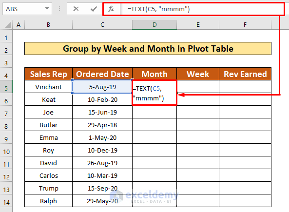
- After typing the formula in Formula Bar, simply press Enter on your keyboard. As a result, you will get the output of the TEXT The return is “August”.

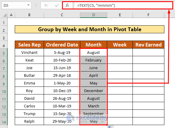
- Hence, AutoFill the TEXT function to the rest of the cells in column D.
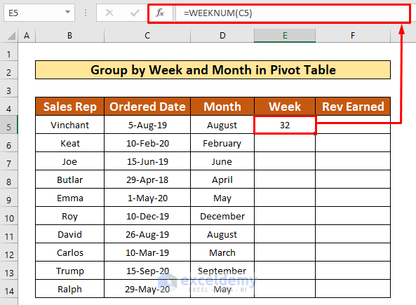
- Now, we will calculate the week number to group by week and month in the pivot table. To calculate the week number, we will apply the WEEKNUM function. To do that, firstly, select cell E5, and type the below WEEKNUM function to calculate the Week number from the corresponding Ordered date. The WEEKNUM function is,
=WEEKNUM(C5)
- Hence, again, press Enter on your keyboard. As a result, you will get the output of the WEEKNUM The output is “32”.
- Further, AutoFill the WEEKNUM function to the rest of the cells in column E.

- After completing the above process, and adding the revenue earned by the sales representatives in column F, we will be able to create our dataset to group the Excel pivot table by week and month.
Step 2: Creating a Pivot Table from Given Dataset in Excel
In this step, we will create a Pivot Table to group by month and week. To do that, let’s follow the instructions below to learn!
- To group the Pivot Table by Week and Month, firstly, select your entire dataset, secondly, from the Insert tab, go to,
Insert → Tables → PivotTable → From Table/Range
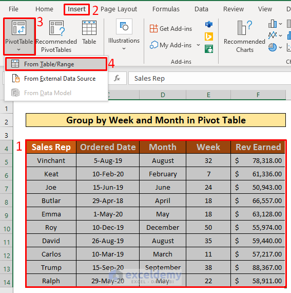
- As a result, a PivotTable from table or range dialog box will appear in front of you. From that dialog box, firstly, type “Overview!SBS4:$F$14” in the Table/Range typing box under Select a table or range Secondly, check the Existing Worksheet. At last, press OK.

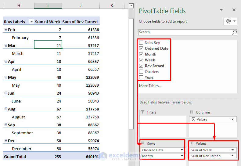
- After completing the above process, you will be able to create a pivot table which has been given in the below screenshot.
Step 3: Grouping by Week and Month in the Pivot Table
After creating the Pivot table, we will group the Pivot Table by week and month. From our dataset, we can easily do that. Let’s follow the instructions below to group by week and month!
- First of all, press right-click on any cell under the Row labels As a result, a window will appear in front of you. From that window, select the Group option.

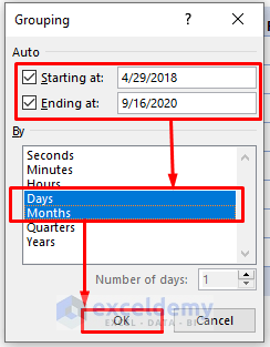
- Hence, a dialog box named Grouping pops up. From the Grouping dialog box, firstly check the Starting at and Ending at Secondly, select Days and Months under the By drop-down list. At last, press OK.
- After completing the above process, you will be able to group the Pivot Table by week and month which has been given in the below screenshot.

Read More: How to Group by Month and Year in Excel Pivot Table
Things to Remember
👉 You can use Ctrl + Alt + F5 to refresh all pivot tables.
👉 To create a Pivot Table, you have to select your entire dataset, secondly, from the Insert tab, go to,
Insert → Tables → PivotTable → From Table/Range
Download Practice Workbook
Download this practice workbook to exercise while you are reading this article.
Conclusion
I hope all of the suitable methods mentioned above to group pivot tables by week and month will now provoke you to apply them in your Excel spreadsheets with more productivity. You are most welcome to feel free to comment if you have any questions or queries.
Related Articles
- How to Group by Year in Excel Pivot Table
- [Fix] Cannot Group Dates in Pivot Table
- [Fixed] Excel Pivot Table Not Grouping Dates by Month
<< Go Back to Group Dates in Pivot Table | Group Pivot Table | Pivot Table in Excel | Learn Excel
Get FREE Advanced Excel Exercises with Solutions!
