In this article, we will demonstrate how to group by year in an Excel Pivot Table.
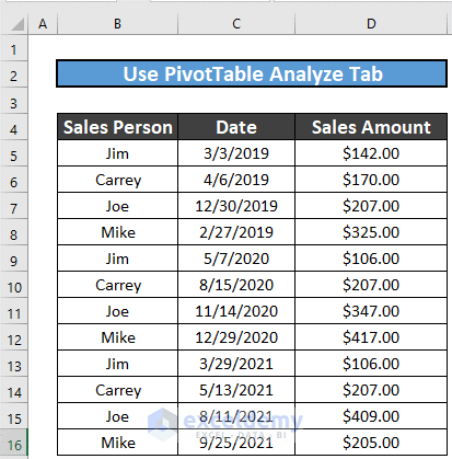
In the dataset below we have some Sales Persons with corresponding Dates and Sales Amounts. We’ll group these dates by year using 3 different techniques.
Method 1 – Using the Pivot Table Fields Feature to Group by Year
The simplest way to group dates in a Pivot Table is to use PivotTable Fields.
Steps:
- Select the entire dataset.
- Go to the Insert tab >> PivotTable >> select From Table/Range.

- In the window that appears, select the range and New Worksheet as the location for the Pivot Table.
- Click OK.

Excel will create a pivot table in a new worksheet.
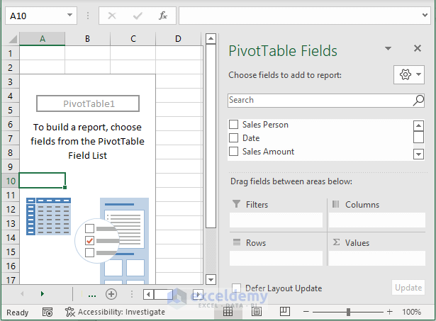
- In the Pivot Table worksheet, select Date and drag it to Rows.
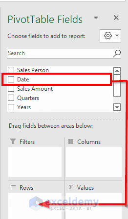
Excel automatically groups the dates.
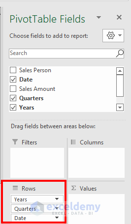
- Similarly, drag Sales Person to the Columns field and Sales Amount to the Values field.
The pivot table will look like this:
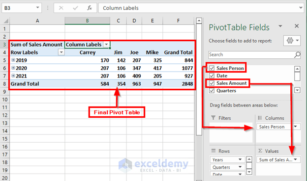
To finish, format the table as you wish.
Read More: How to Group by Week in Excel Pivot Table
Method 2 – Using the Pivot Table Analyze Tab to Group Dates by Year
Another way of grouping dates by year in a Pivot Table is by applying the PivotTable Analyze tab,
Steps:
- Create a pivot table following Method 1.
The table will look like this:

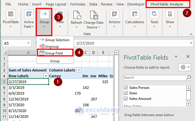
- Select any date.
- Go to the PivotTable Analyze tab.
- Select Group >>Group Field.
A new box named Grouping will pop up.
- Select Years.
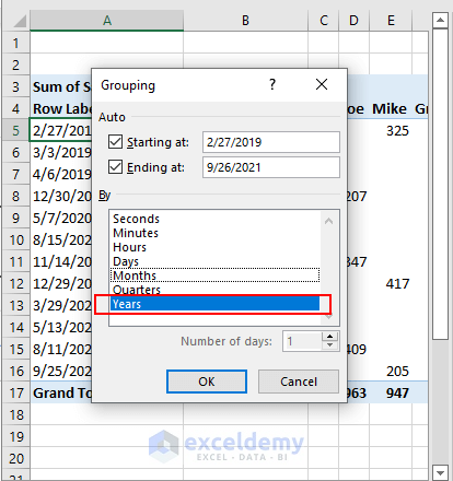
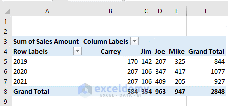
Excel will group the dates by year.
Read More: How to Group by Month in Excel Pivot Table
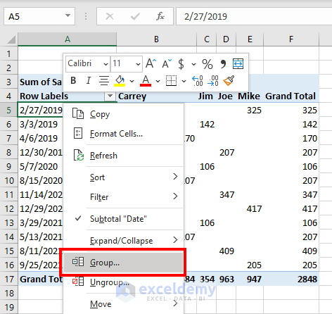
Method 3 – Using the Context Menu to Group by Year in a Pivot Table
We can also use the context menu to group dates by year.
Steps:
- Create a pivot table following Method 1.
The table will look like this:

- Select any date and right-click your mouse to bring up the context menu.
- Select Group.
A new box named Grouping will pop up.
- Select Years.

Excel will group the dates by year.

Things to Remember
- Method 1 works for Excel version 2016 and later.
- If you use earlier versions, use Method 2 and Method 3.
Download Practice Workbook
Related Articles
- How to Group by Week and Month in Excel Pivot Table
- How to Group by Month and Year in Excel Pivot Table
- [Fix] Cannot Group Dates in Pivot Table
- [Fixed] Excel Pivot Table Not Grouping Dates by Month
<< Go Back to Group Dates in Pivot Table | Group Pivot Table | Pivot Table in Excel | Learn Excel
Get FREE Advanced Excel Exercises with Solutions!
