In this article, we’ll demonstrate various examples of how to use the WEEKNUM function effectively in Excel.

Introduction to the WEEKNUM Function in Excel
- Function Objective
The WEEKNUM function is used to calculate the week number of a date.
- Syntax
=WEEKNUM(serial_number, [returns_type])

- Arguments Explanation
| Arguments | Required/Optional | Explanation |
|---|---|---|
| serial_number | Required | Value from which to calculate the week number |
| returns_type | Optional | From which day the week begins |
The WEEKNUM function can be used in two different [returns_type] ways:
System 1: Week 1 specifies the week which contains January 1st;
System 2: Week 1 is the week that includes the first Thursday of the year.
| Returns_type | Week begins on | System |
|---|---|---|
| 1 or omitted | Sunday | 1 |
| 2 | Monday | 1 |
| 11 | Monday | 1 |
| 12 | Tuesday | 1 |
| 13 | Wednesday | 1 |
| 14 | Thursday | 1 |
| 15 | Friday | 1 |
| 16 | Saturday | 1 |
| 17 | Sunday | 1 |
| 21 | Monday | 2 |
How to Use Excel WEEKNUM Function: 5 Examples
To illustrate our examples, we’ll use the following dataset of a garden maintenance schedule.

We have used the Microsoft Excel 365 version in this article; but you may use any other version at your convenience. Please leave a comment if any part of this article does not work in your version.
Example 1 – Use Text as Argument of WEEKNUM Function to Calculate Week Number
The WEEKNUM function can take valid text as an argument, meaning a date, and return the corresponding week number for this date.
STEPS:
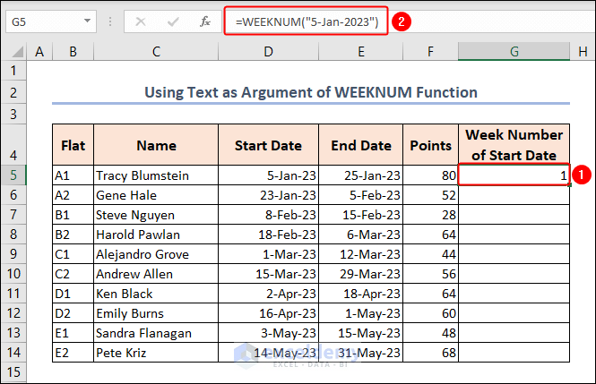
- In cell G5, enter the following formula and press ENTER:
=WEEKNUM("5-Jan-2023")It returns 1 as the date is in the first week of the year.
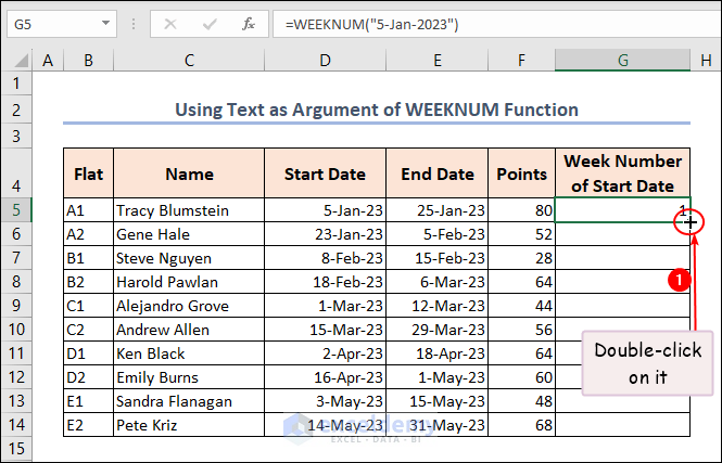
- Bring the cursor to the right-bottom corner of cell G5 and it’ll look like a plus (+) sign. It’s the Fill Handle tool.
- Double-click on the Fill Handle to AutoFill the remaining cells in Column G.
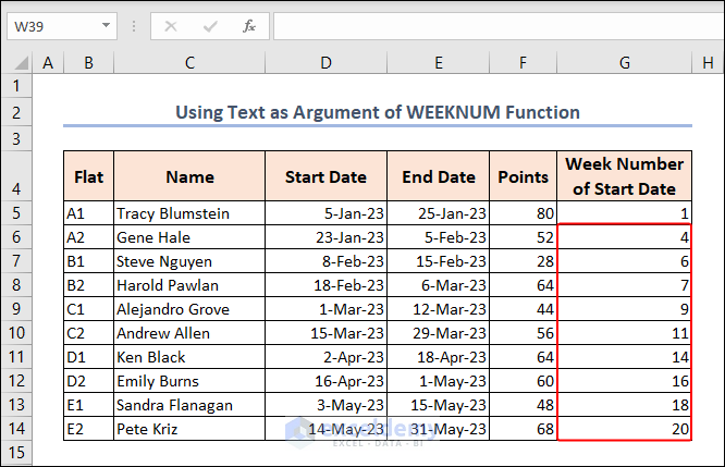
The final output is as follows:
Example 2 – Use Cell Reference as Argument to Find Week Number in Excel
We can achieve the same output using a cell reference instead of a date string as an argument in the WEEKNUM function.
STEPS:
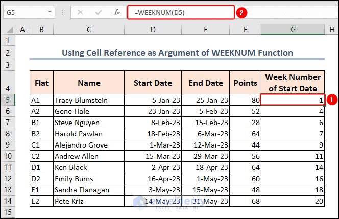
- Enter the following formula in cell G5 and press ENTER:
=WEEKNUM(D5)It confirms that this start date (5-Jan-2023) is in the first week of the year 2023.
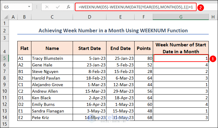
Example 3 – Return Week Number in a Month
Combine the WEEKNUM, DATE, and MONTH functions to convert a specific date to its corresponding week number within the month.
STEPS:
- Enter the following formula in cell G5:
=WEEKNUM(D5)-WEEKNUM(DATE(YEAR(D5),MONTH(D5),1))+1Formula Breakdown
- WEEKNUM(D5): Calculates the week number for the date in cell D5, based on the default week numbering system in Excel.
- DATE(YEAR(D5),MONTH(D5),1): Constructs a new date using the year and month from the date in cell D5 and a day of 1. It represents the first day of the same month as the date in cell D5.
- WEEKNUM(DATE(YEAR(D5),MONTH(D5),1)): Calculates the week number for the constructed date above, based on the default week numbering system in Excel.
- WEEKNUM(D5)-WEEKNUM(DATE(YEAR(D5),MONTH(D5),1)): Subtracts the week number just obtained from the week number obtained in step 1, returning the difference in week numbers between the specific date in cell D5 and the first day of the same month.
- WEEKNUM(D5)-WEEKNUM(DATE(YEAR(D5),MONTH(D5),1))+1: Adds 1 to the difference calculated in step 4. The purpose is to adjust the week number difference to account for the starting week.
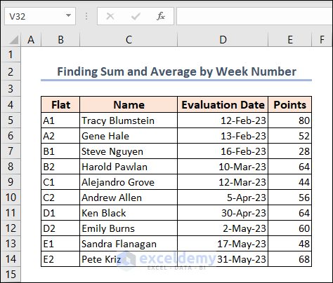
Example 4 – Find Sum and Average by Week Number in Excel
We can also use week numbers for other types of calculations. To demonstrate, we expand our dataset to include the Evaluation Date column – the date when the performance of each person will be evaluated – where we’ll use the Weeknum function to compute the sum of points as well as the average points in a week.
STEPS:
- To find the Week Number of the corresponding Evaluation Date, the formula in cell F5 is the following:
=WEEKNUM(D5)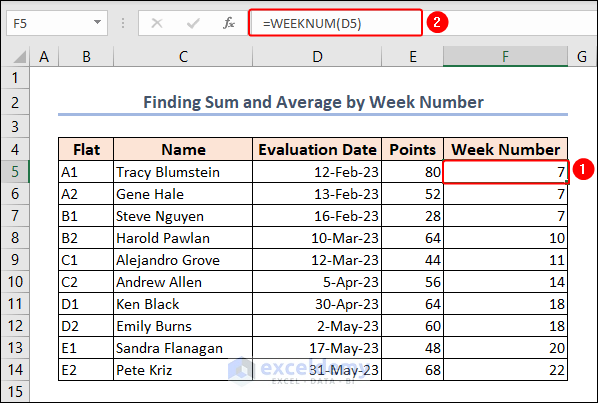
- To detect the unique week numbers from Column F, the formula in cell B17 is as follows:
=UNIQUE(F5:F14)The UNIQUE function returns a list of unique values in a range or in a list.
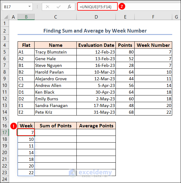
- To calculate the sum of points in week 7, insert the following formula in cell C17:
=SUMIF($F$5:$F$14,B17,$E$5:$E$14)The SUMIF function adds the cells specified by a given condition or criteria.
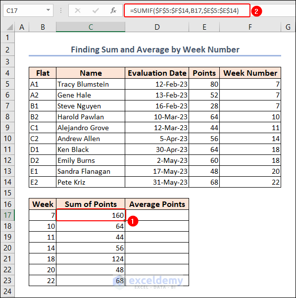
The sum of points for Week 7 is 160 (cell C17), which is the sum of points in the E5:E7 range.
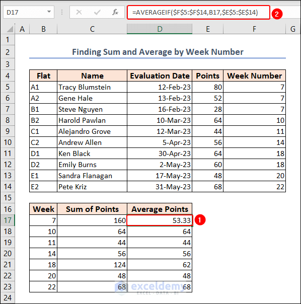
- Input the following formula in cell D17 to get the Average Points for this month:
=AVERAGEIF($F$5:$F$14,B17,$E$5:$E$14)The AVERAGEIF function finds the average for the cells specified by a given condition or criteria.
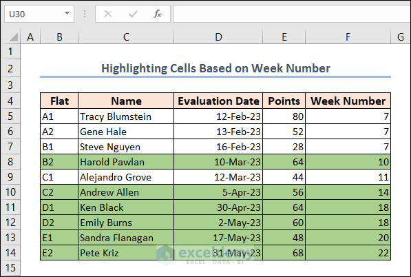
Example 5 – Highlight Cells Based on Week Number Using WEEKNUM Function
We can highlight cells based on week numbers by using the WEEKNUM and MOD functions together. Say we want to highlight rows in which Evaluation Date appears in an even week number.
STEPS:
Calculate the Week Number using the following function in Column F:
=WEEKNUM(D5)
- Select the B5:F14 range.
- Go to the Home tab >> Conditional Formatting on the Styles group >> New Rule.
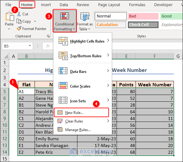
The New Formatting Rule dialog box opens.
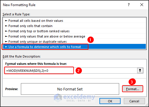
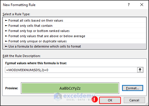
- Click on Use a formula to determine which cells to format in the Select a Rule Type section.
- In the Format values where this formula is true: box, enter the following formula:
=MOD(WEEKNUM($D5),2)=0- Click Format.
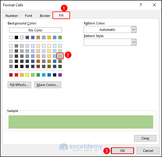
- In the Format Cells dialog box, go to the Fill tab.
- Select your desired color and click OK.
A preview of the formatting is shown.
- Click OK.
Excel highlights rows that have Evaluation Date in an even week number. To verify, check against the value in Column F.
[Fixed!] WEEKNUM Is Not Working in Excel: Reason with Solution
Sometimes, we face errors while working with the WEEKNUM function. In the following image, we get #NUM! and #VALUE! errors. But why?
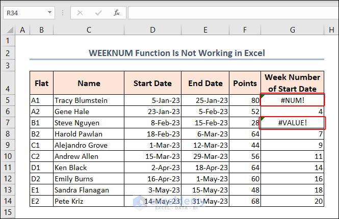
- We used 18 as the return_type argument of this function, which is not valid. Hence the error.
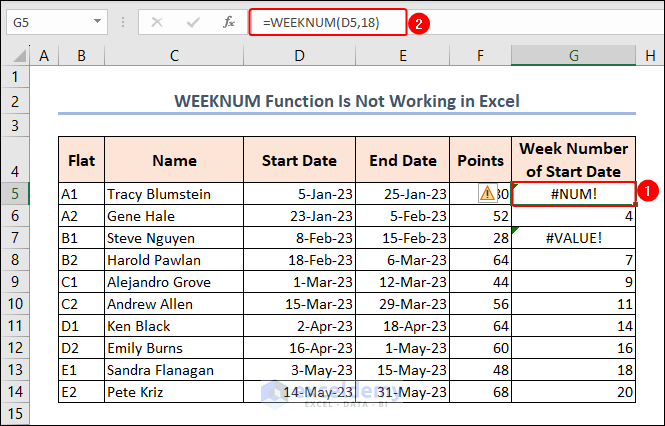
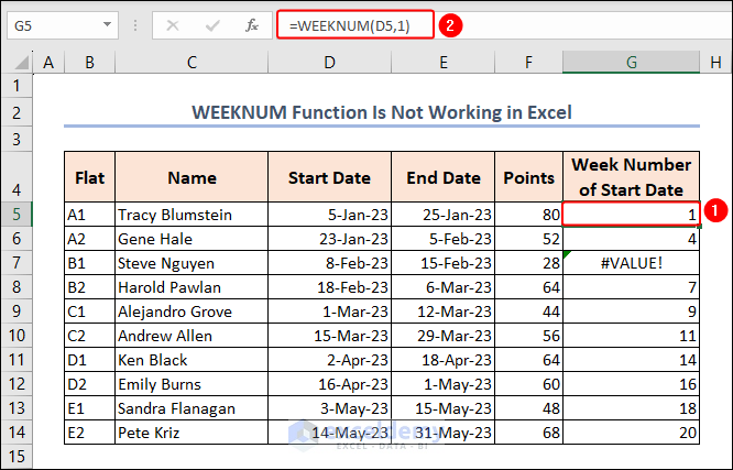
- Change the formula in cell G5 to the following:
=WEEKNUM(D5,1)Now it returns the correct output.
- We will also get errors when we use invalid dates. For example, we used 29 Feb in the below image, a date which doesn’t exist in 2023.
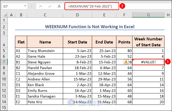
- Correct the formula in cell G7 to the following:
=WEEKNUM(“28-Feb-2023”)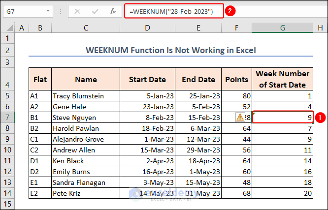
The error is gone and the function is working correctly.
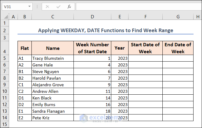
How to Find Week Range Using WEEKDAY & DATE Functions in Excel
Say we want to determine the Start Date and End Date of the corresponding Week in Column D.
To illustrate this process, we add a new column Weeks in Between Dates to our dataset. 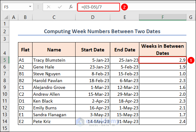
- Use the following formula in cell F5 to find the Start Date of the Week:
=DATE(E5,1,-2)-WEEKDAY(DATE(E5,1,3))+D5*7Formula Breakdown
- DATE(E5, 1, -2): Constructs a date using the year from cell E5, a month of 1 (January), and a day of -2. By using -2, it sets the date to the second-to-last day of the previous month (December of the specified year).
- WEEKDAY(DATE(E5, 1, 3)): The WEEKDAY function calculates the weekday number for the specified date, which is the 3rd day of January in the year specified in cell E5.
- DATE(E5,1,-2)-WEEKDAY(DATE(E5,1,3)): Subtracts the weekday value (obtained in step 2) from the constructed date in step 1. The purpose is to obtain the date of the first day of the week that contains January 1st in the specified year.
- D5*7: Multiplies the value in cell D5 by 7, which represents the number of weeks. This calculates the total number of days to add to the date obtained in step 3.
- DATE(E5,1,-2)-WEEKDAY(DATE(E5,1,3))+D5*7: The date obtained in step 3 is added to the total number of days calculated in step 4. This results in the desired week’s date.
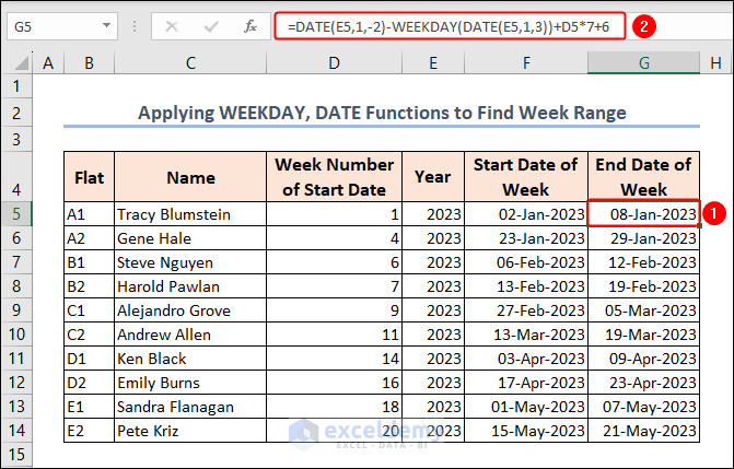
- The formula (in cell G5) we use to find the End Date of Week is the following:
=DATE(E5,1,-2)-WEEKDAY(DATE(E5,1,3))+D5*7+6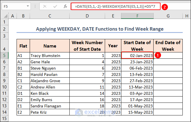
How to Compute Week Numbers Between Two Dates in Excel
It is also possible to determine the number of weeks between the two dates.
STEPS:
=(E5-D5)/7We divide the difference between the Start and End dates by 7 as there are 7 days in a week.
Read More: How to Convert Date to Week Number of Month in Excel
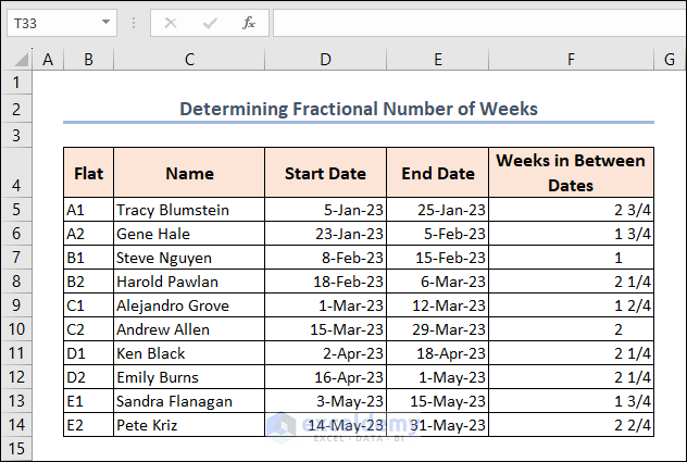
How to Determine Fractional Number of Weeks in Excel
We can return the number of weeks between two dates in fractional as opposed to decimal format.
STEPS:
- Insert the same formula in cell F5 as the previous example.
- Select the F5:F14 range and press CTRL + 1 on your keyboard.
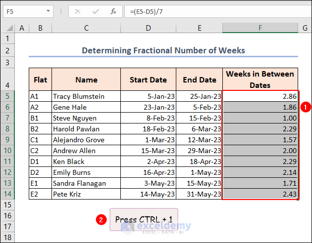
- Select Number >> Fraction >> As quarters (2/4).
- Click OK.
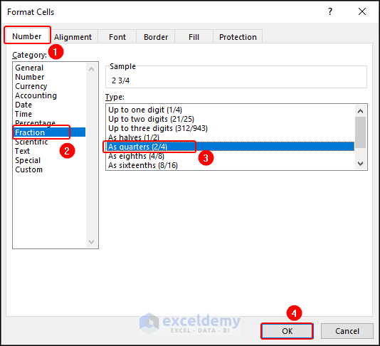
The output in fractional format is returned.
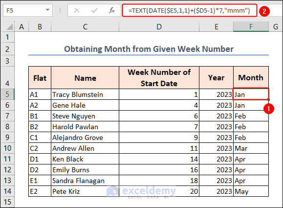
How to Obtain Month from Given Week Number in Excel
STEPS:
- Enter the following formula in cell F5:
=TEXT(DATE($E5,1,1)+($D5-1)*7,"mmm")The TEXT function returns a numeric value in a specified format.
Formula Breakdown
- DATE($E5, 1, 1): Constructs a date using the year from cell E5, a month of 1 (January), and a day of 1. This creates the first day of the specified year.
- ($D5-1)*7: 1 is subtracted from the value in cell D5 (week number), and then the result is multiplied by 7. This calculates the number of days to add to the first day of the year to reach the desired week.
- The result of step 2 is added to the date obtained in step 1. This provides the date of the desired week.
- TEXT(…, “mmm”): The final step involves formatting the resulting date as an abbreviated month name. The TEXT function is used to convert the date into the desired format.
Things to Remember
- #VALUE! error occurs when we use non-numeric data or data that is not a valid date.
- #NUM! error occurs when the function does not permit the value or the data is numeric but out of range.
- Ensure that the dates you provide to the WEEKNUM function are in a valid format recognized by Excel, such as proper date values or valid date serial numbers.
- Take note of any cultural or regional differences in week numbering systems when using the WEEKNUM function, as different countries may have variations in their week numbering conventions.
Frequently Asked Questions
1. Can I use the WEEKNUM function in combination with other functions or formulas?
Yes.
2. Can I adjust the WEEKNUM function to consider Monday as the first day of the week?
Yes, by adding an optional second argument with a value of 2.
3. Can the WEEKNUM function handle dates from different years?
Yes, it accurately calculates the week number based on the specified date, regardless of any transition between years.
4. Does the WEEKNUM function consider leap years when calculating week numbers?
Yes, it adjusts the week numbers accordingly based on an additional day in a leap year.
Download Practice Workbook
<< Go Back to Excel Functions | Learn Excel
Get FREE Advanced Excel Exercises with Solutions!

How to get weeknumber and the year it falls into from a date … e.g. special cases for dates that fall into a week say, week #53.
The for 1-January-2027 should be 2026w53 and not 2027w53 !!
[ ISO weeknumber format // System 2 ]
Hello Blemish Go,
To get the ISO week number and the correct year (so that 1-Jan-2027 is shown as 2026w53), you need to follow the ISO 8601 standard. Excel’s built-in WEEKNUM function alone won’t handle the year rollover correctly for ISO weeks, but you can use the ISOWEEKNUM function (available in Excel 2013 and later) plus an extra formula for the ISO year.
Steps:
Week Number:
Use =ISOWEEKNUM(A1) where your date is in cell A1.
ISO Year:
Use this formula for the ISO week year (paste in any cell):
=A1-WEEKDAY(A1,2)+4
Then extract the year from that result:
=YEAR(A1-WEEKDAY(A1,2)+4)
Combine both for the ISO format:
=YEAR(A1-WEEKDAY(A1,2)+4) & “w” & TEXT(ISOWEEKNUM(A1),”00″)
For 1-Jan-2027, this will correctly return 2026w53.
Regards
ExcelDemy