How to Use Excel MONTH Function: 6 Methods

Method 1 – Simply Use Excel MONTH Function to Get the Month Number

Steps:

• Type the below formula in Cell C5.

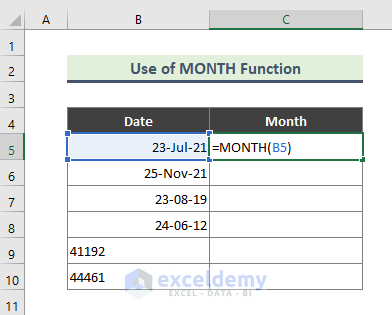
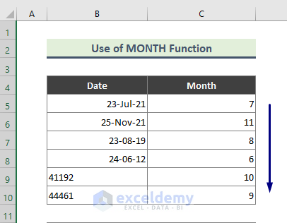
• The month number regarding the dates will be shown as output. Use Fill Handle (+) to copy the formula to the rest of the cells.

Note:

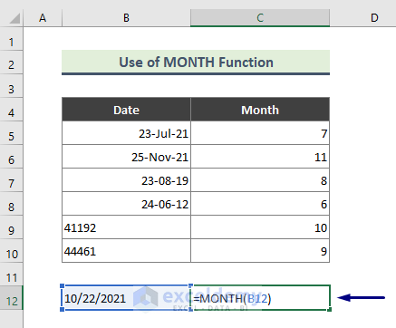
➤ If you do not provide an invalid date format, the MONTH function will return an error. For instance, ‘10/22/2021’ is an invalid date. See the outcome of applying the MONTH function to it.

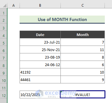
➤ Here is the error (#VALUE!) returned by the MONTH function.

Method 2 – Combination of MONTH & DATE Functions in Excel

Steps:

• Type the following formula in Cell C5.

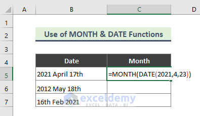
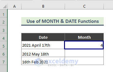
The DATE function converts the improper date value to a recognizable format. The MONTH function extracts the month number from the date.

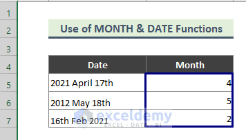
• You will get the following result.

• You can find months of other improper dates too.

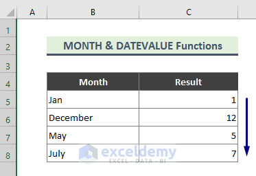
Method 3 – Apply MONTH and DATEVALUE Functions Converting Month Value to Number

Steps:

• Type the below formula in Cell C5.

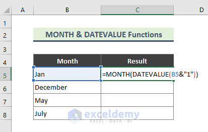
The DATEVALUE function converts a date in the form of text to a number that represents the date in Microsoft Excel date-time code. DATEVALUE(B5&”1”) returns ‘36892’. Finally, the MONTH function extracts the month value from ‘36892’.

• Get the following result.

Method 4 – Excel MONTH and YEAR Functions Combination

Steps:

• Type the below formula in Cell D5.

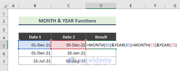
• The following will be the outcome.

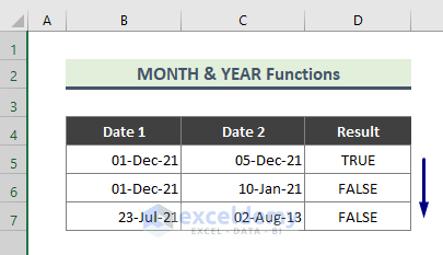
How Does the Formula Work?

➨ MONTH(B5)

The MONTH function extracts the month number ‘12’.

➨ YEAR(B5)

The YEAR function returns the year of ‘01-Dec-21’, which is ‘2021’.

➨ MONTH(B5)&YEAR(B5)=MONTH(C5)&YEAR(C5)

This formula matches both the dates and returns ‘TRUE’.

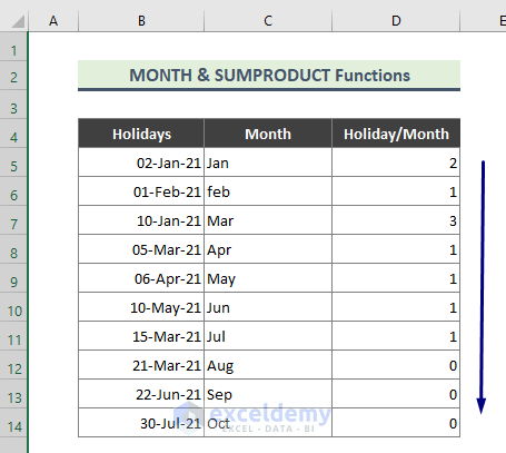
Method 5 – Use MONTH Function with SUMPRODUCT Function

Steps:

• Type the below formula in Cell D5.

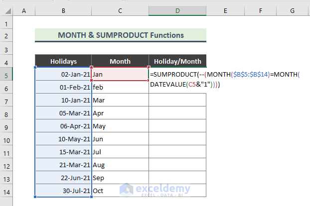
• You will get the holidays month-wise.

How Does the Formula Work?

➨ MONTH($B$5:$B$14)

This part of the formula will return the month number of the range B5:D14.

{1,2,1,3,4,5,3,3,6,7}

➨ MONTH(DATEVALUE(C5&”1″))

This part will return the number value of the month of Cell E4.

➨ SUMPRODUCT(–(MONTH($B$5:$B$14)=MONTH(DATEVALUE(C5&”1″))))

This formula will match the month given from MONTH(B5:B14) with the result of MONTH(DATEVALUE(C5&”1″)) and add 1 when the result is matched.

Method 6 – Apply MONTH and CHOOSE Functions Combination in Excel

Steps:

• Type the below formula in Cell C5.

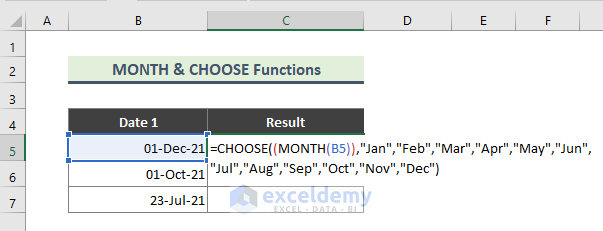
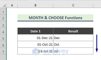
• Get the month name (in ‘mmm’ format). Use Full Handle (+) to copy the formula to the rest of the cells.

How Does the Formula Work?

➨ MONTH(B5)

This part of the formula will return ‘12’.

➨ CHOOSE((MONTH(B5)),”Jan”,”Feb”,”Mar”,”Apr”,”May”,”Jun”,”Jul”,”Aug”,”Sep”,”Oct”,”Nov”,”Dec”)

The CHOOSE function chooses a value or action to perform from a list of values, based on an index number. This formula will choose ‘Dec’ from the list as the result of the previous part of the formula is ‘12’.

Download the Practice Workbook

You can download the practice workbook that we have used to prepare this article.

Excel MONTH Function: Knowledge Hub

<< Go Back to Excel Functions | Learn Excel