Method 1 – Grouping Data by Month Automatically
Step 1 – Create a Pivot Table
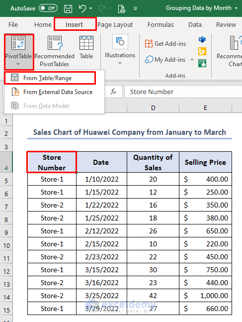
- Select the entire dataset.
- Click on the Insert ribbon at the top.
- Select the From Table/Range option from the PivotTable drop-down menu.
- You can select the following options from the dialog box. If you selected the table, it should be inserted by default.
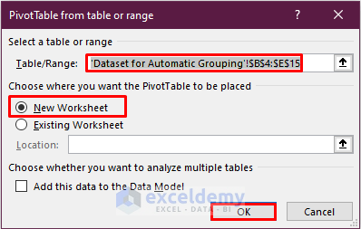
- Click OK.
Step 2 – Group the Data by Month
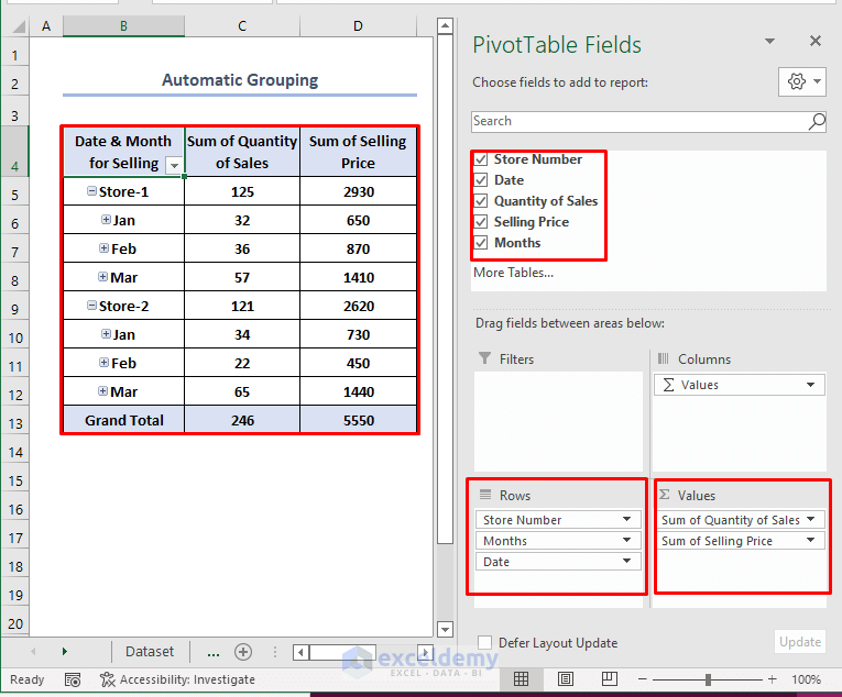
- Drag the Store Numbers, Months, and Dates into Rows and the Sales and Quantities in the Values fields.
- Rename the table headers in the formula bar as Date & Month of Selling like below.
Case 1.1 – Grouping Data by Month Manually
Steps:
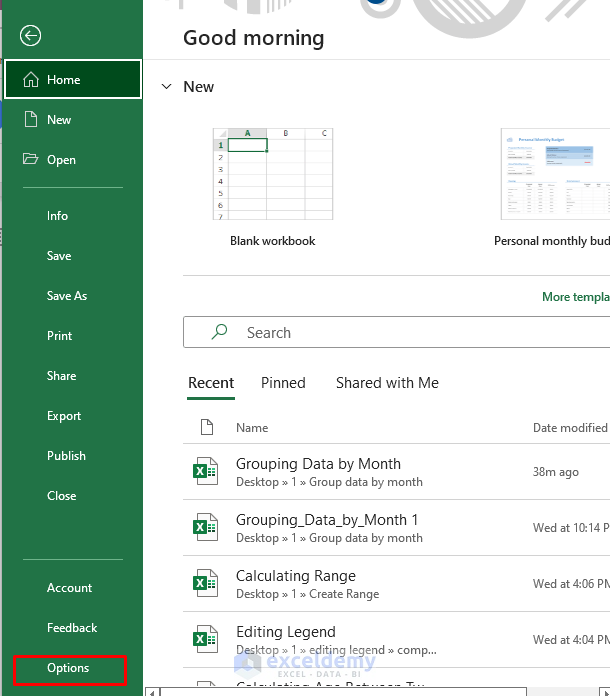
- Select File from the top menu.
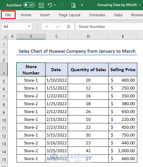
- Go to Options at the bottom.
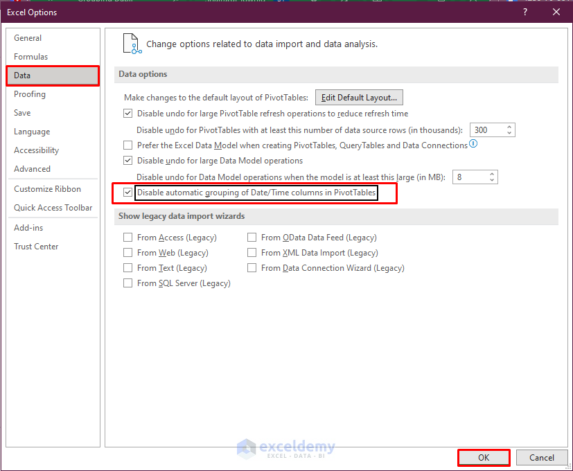
- Choose the Data tab and tick the box next to “Disable automatic grouping of Date/Time columns in PivotTables”.
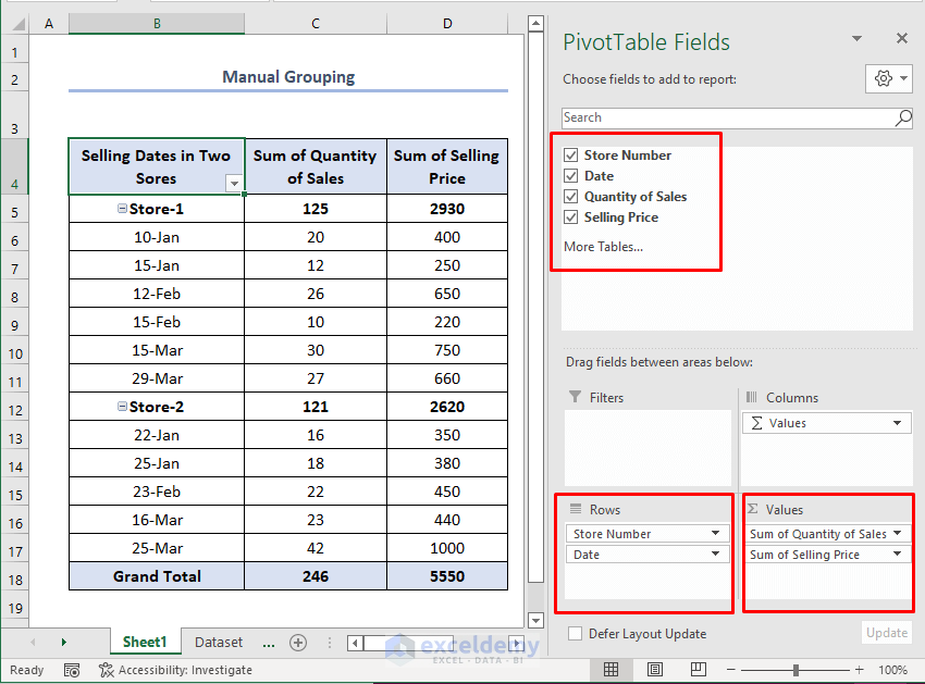
- Insert a PivotTable.
- Drag the objects into the appropriate fields, as shown in the screenshot below.
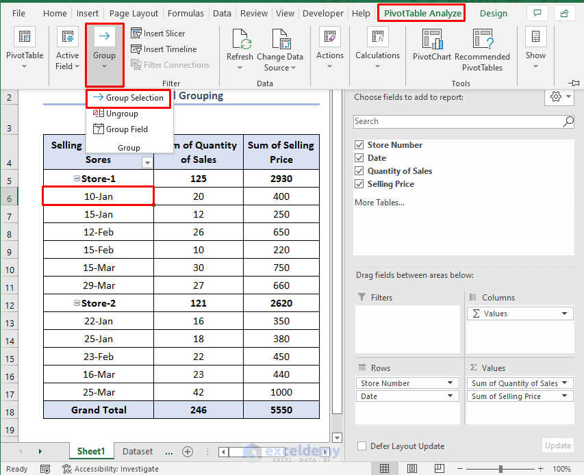
- Choose a Date. We used 10-Jan.
- Pick Group Selection from the drop-down menu on the PivotTable Analyze ribbon.
- The start date (Starting at), end date (Ending at), and grouping (By) options are then presented in a box as shown below.
- Choose Months to group data by month and click OK.
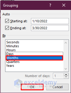
- Here’s the output.

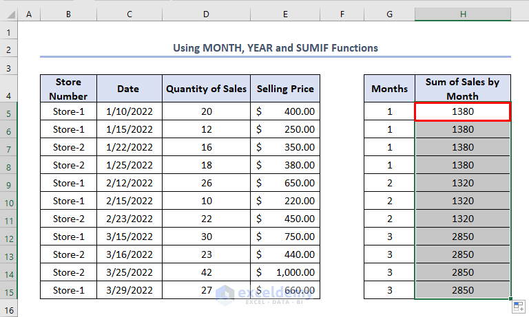
Method 2 – Grouping Data by Month by Combining Excel Functions
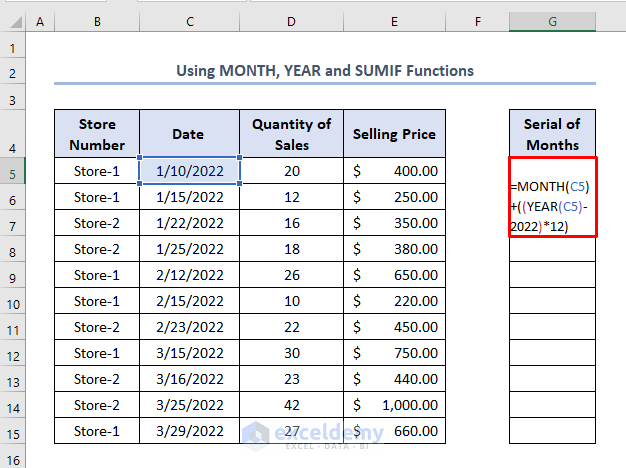
- Insert the following formula in G5:
=MONTH(C5)+((YEAR(C5)-2022)*12)C5 refers to the date which the serial needs to calculate.
The MONTH (C5) function takes the value of the month from the C5 cell. It is 1. YEAR(C5) function takes the year’s value from the C5 cell. It is 2022. The output is subtracted by 2022 by the argument YEAR(C5)-2022. This output is zero. Then it is multiplied by 12. The whole formula MONTH (C5)+((YEAR(C5)-2022)*12) gives the output 1.
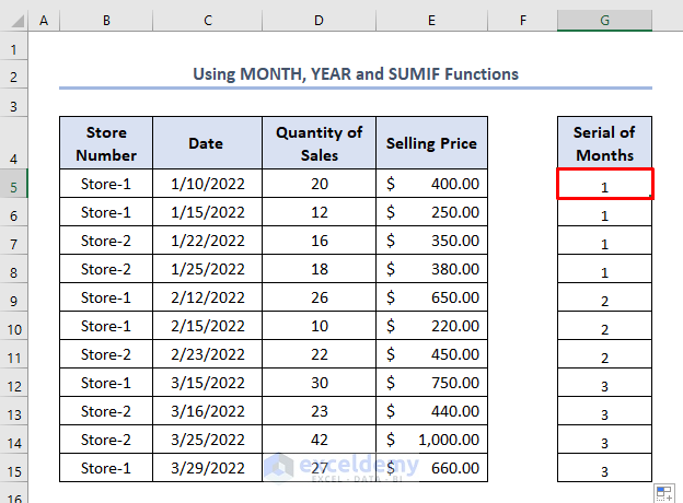
- After clicking Enter, you’ll get the output as the serial number of the month in the date from column C.
- By using the Fill Handle from cells G6 to G15, you’ll get all the results for the helper column.
- Put the following formula in the H5 cell.
=SUMIF($G$5:$G$15,G5,$E$5:$E$15)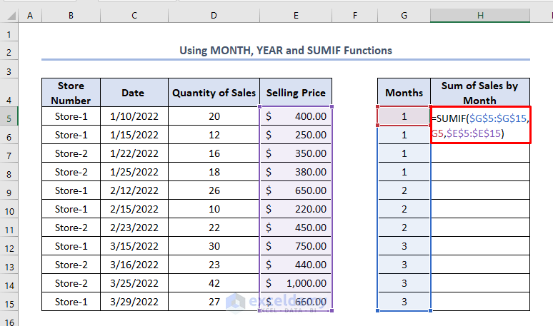
- Press Enter and AutoFill by double-clicking the Fill Handle.
- Remove duplicate values from the helper column by whatever method you prefer to clean up the table.
Download the Practice Workbook
Related Articles
- Excel Pivot Table Group by Week (3 Suitable Examples)
- How to Group Dates in Excel Chart (3 Easy Ways)
- [Fix] Cannot Group Dates in Pivot Table: 4 Possible Solutions
- How to Group Dates in Pivot Table (7 Ways)
- How to Group by Year in Excel Pivot Table (3 Easy Methods)

