When generating a Pivot Table in Excel, various Field Buttons including Filter Arrows appear automatically on the table headers. In this article, we will demonstrate 3 ways to hide these Filter Arrows from a Pivot Table in Excel.
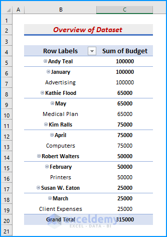
The first two methods are straightforward and use basic Excel features, while the third involves applying VBA code to our file To illustrate our methods, we’ll use the following dataset that represents a company budget list, implemented in a Pivot Table. The Row Labels header in column B containing Filter Arrows is able to perform sorting and filtering for the specific column.
Method 1- Using the Field Headers Feature to Hide Filter Arrows from a Pivot Table in Excel
This quick and simple method will completely hide the Filter Arrows in no time. However, the Field Names will also disappear.
Steps:
- Click anywhere on the Pivot Table.
- Go to PivotTable Analyze and click on Field Headers in the Show group.
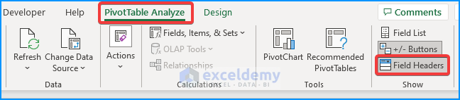
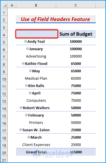
The Filter Arrow along with Field Name disappears.
- Display the Filter Arrow again by clicking the Field Headers option again.
Method 2 – Unchecking the Display Field Caption and Filter Drop Downs to Remove Filter Arrows
The second method will access the PivotTable Options to completely hide all headings and arrows. This is particularly useful if we want to restrict users’ ability to choose items from one or more header drop-down icons after setting up a Pivot Table.
Steps:
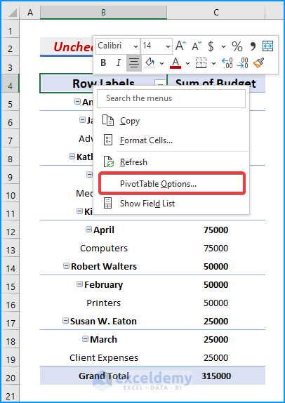
- Right-click on the Pivot Table.
- From the context menu, select PivotTable Options.
The PivotTable Options dialog box slides into view.
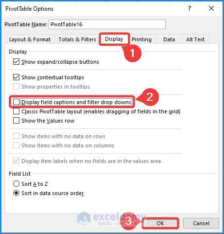
- Click the Display option.
- Uncheck the Display field captions and filter drop downs box.
- Click OK to close the dialog box.
The Filter Arrows disappear from the table headings.
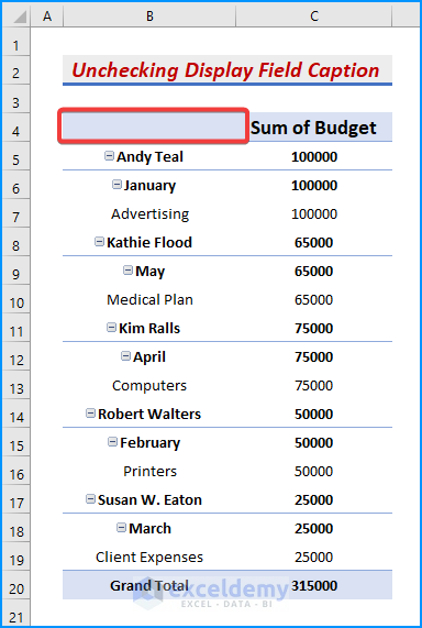
Although the previous methods are quick and simple, they may not be the best options, since without Field Names or Header Names, it might not be obvious what data the report is showing.
Method 3 – Running an Excel VBA Code to Hide Filter Arrows in a Pivot Table
We can run some VBA code to remove the Filter Arrows from Pivot Table headers while leaving the Field Names intact.
Steps:
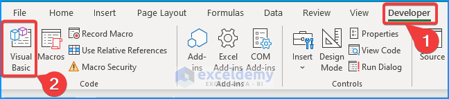
- Go to the Developer tab and click Visual Basic. Or press ALT + F11.
The Visual Basic window pops up.
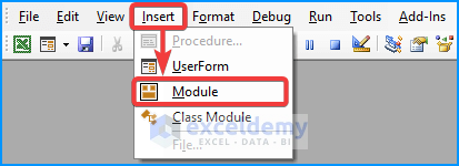
- Click Insert and then Module to open a module box.
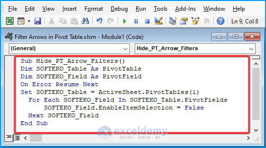
- In the module box, enter the following VBA code:
Sub Hide_PT_Arrow_Filters()
Dim SOFTEKO_Table As PivotTable
Dim SOFTEKO_Field As PivotField
      On Error Resume Next
Set SOFTEKO_Table = ActiveSheet.PivotTables(1)
      For Each SOFTEKO_Field In SOFTEKO_Table.PivotFields
      SOFTEKO_Field.EnableItemSelection = False
Next SOFTEKO_Field
End Sub
This code will hide all the arrows. We can use .RowFields or .ColumnFields instead of the .PivotFields object to hide individual arrows in the header.
- Save the code and close the window.
- Back in the active sheet, go to the Developer tab again and click Macros.
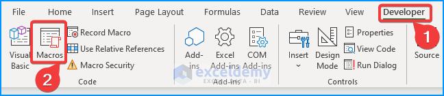
The Macro dialog box pops up.
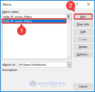
- Select the Macro Name and click Run.
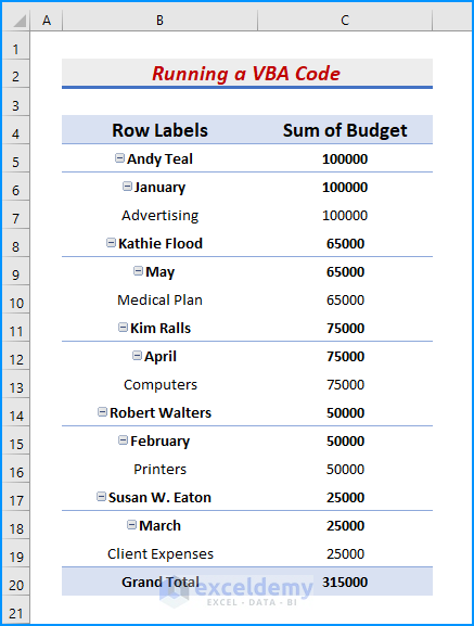
The Filter Arrows on the table headers are removed completely.
Read More: Excel Pivot Table Filter Based on Cell Value
Download Practice Workbook
<< Go Back to Pivot Table Filter | Pivot Table in Excel | Learn Excel
Get FREE Advanced Excel Exercises with Solutions!
