Latest Posts From Yousuf Khan

Here's a simplified overview of data mining in a smaller dataset. Download the Practice Workbook Data Mining Excel Example.xlsx How to ...

Method 1 - Merge Multiple Data Sources in One Query with Power Query Step 1: Import Data into Excel Workbook Import an Excel workbook from the Source ...

Power Query Excel: Knowledge Hub How to Use Power Query Date Functions in Excel Power Query Multiple Sources in One Query Power Query Get Data from ...

Power Query Joins: Knowledge Hub Combine Two Tables Using Power Query in Excel How to Perform Left Join in Excel Perform Left Outer Join in Excel ...

This is an overview: Download Practice Workbook Download the practice workbook. Data Analysis ToolPak in Excel.xlsx The Data ...

Pivot Table Calculations: Knowledge Hub Difference in Pivot Table Pivot Table Count Pivot Table Running Total Subtotals in Pivot Table Pivot ...

This is an overview. Download Practice Workbook Download the practice workbook. Linking in Excel.xlsx Absolute vs Relative Linking ...

Pivot Table Grand Total: Knowledge Hub How to Show Grand Total in Pivot Table How to Collapse the Table to Show the Grand Totals Only Pivot Table ...

Subtotals within pivot tables are a pivotal feature that enhances the way you analyze and summarize data, providing a comprehensive view of aggregated ...

Pivot Table Running Total: Knowledge Hub How to Use Pivot Table to Calculate Running Total by Date in Excel << Go Back to Pivot Table ...

Introduction to Extensible Markup Language (XML) XML, a markup language similar to HTML, is specifically designed to store and transport data. Here are some ...

Pivot Table Count: Knowledge Hub Count Rows in Group with Pivot Table in Excel How to Count Unique Values Using Excel Pivot Table << Go ...

Difference in Pivot Table: Knowledge Hub Excel Pivot Table: Difference Between Two Columns Pivot Table: Percentage Difference between Two Columns ...
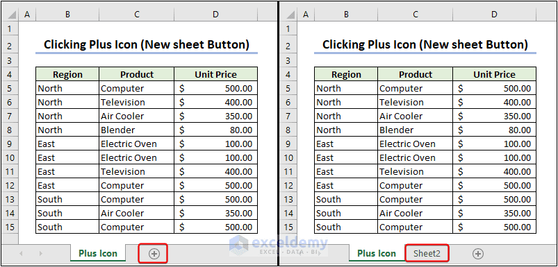
Download the Practice Workbook Insert New Worksheet.xlsm How to Insert a New Worksheet in Excel Method 1 - Clicking the Plus Icon (New Sheet ...
In this article, we will discuss the context menu (or right-click menu) in Excel, including 2 ways to open the context menu, how to add and remove commands ...
- 1
- 2
- 3
- …
- 5
- Next Page »
See Our Reviews at


Dear BZOIRO,
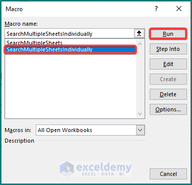
Yes, you can modify the SearchAll function in the given VBA code to search for each word in the cells separately. I have added the modified code in the Excel file below. This modification splits the search value into words using the Split function and loops through each word to find it in the range. If all words are found, the function merges the found ranges into a single range and thoroughly returns it. If any of the words are not found, the function exits and returns Nothing. Here’s how to use this for your case:
1. Initially, assign Macro “SearchMultipleSheetsIndividually” in the Search command box and click Run.
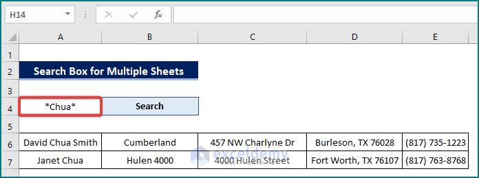
2. Afterward, type the word you wish to look for. Also, don’t forget to use the Wildcards (*, ? etc) while searching. For instance, if you wish to look for a cell of 3 words and has “Emily” in the middle, type *Emily* and then perform searching. Alternatively, if it happens to be the first word, try Emily*.
Download the Excel file to get the modified VBA code and practice by yourself. I hope it works for you.
https://www.exceldemy.com/wp-content/uploads/2023/01/Search-Box-for-Multiple-Sheets.xlsm
Best Regards,
Yousuf Khan (ExcelDemy Team)
Dear LUNDER,
My understanding of your statement implies that there is an issue with the calculations being performed in Microsoft Excel, specifically with the trigonometric functions cosine (cos), cosine (cos), and sine (sin) for certain angle values.
Further, I concur that the error seems to affect the precision of the results starting from the 17th decimal place, which makes the calculated values for the angles cos 90°; cos 270°; sin 180° to be inaccurate. However, it is important to note that the internal representation of floating-point numbers in computers can lead to inaccuracies, especially when working with very small or large numbers, or when performing multiple mathematical operations.
In these cases, you can take the following steps to resolve this issue.
1. Use the RADIANS function to convert the angle from degrees to radians before evaluating the trigonometric functions.
2. Increase the number of decimal places used in the calculations by using the ROUND or ROUNDUP functions.
Best Regards,
Yousuf Khan (ExcelDemy Team)
Dear TONY,
It’s possible that the delay is due to the amount of data being processed by the validation formula. To reduce the delay, you can try the following:
1. Turn off screen updating and calculation during the execution of the macro to reduce the time it takes to display the changes.
2. Consider using a different method for data validation, such as using a custom function or a Macro.
As requested, I have added a revised version of the VBA code with the optimizations under Private Sub Worksheet_Change in Module 3. I hope, these modifications will improve the performance of the code, as it minimizes the amount of visual updates that occur during the process. This will reduce the amount of time it takes for the changes to be made in the sheet as you type in. Download the Excel file and use the desired code.
https://www.exceldemy.com/wp-content/uploads/2023/01/Multiple_Selection_from_Drop-Down.xlsm
Best Regards,
Yousuf Khan (ExcelDemy Team)
Hello ASRA,
The Data Type option in the Data tab in Microsoft Excel is available in both the online and offline versions of Excel.
The offline version of Microsoft Excel is part of the Microsoft Office suite, which can be purchased and installed on your computer. Once you have installed Microsoft Office, you can access Microsoft Excel from the start menu or by double-clicking on an existing Excel file on your computer. The Data Type option in the Data tab will be available in the Excel application after installation. I hope this helps.
Regards,
Yousuf Khan (ExcelDemy Team)
Dear GORAN ZORIC,
Thank you for your comment! We are glad you took the time to review the article. Regarding the trade direction (BUY or SELL), it is actually represented in the Long / Short (L/S) column in the trading journal template. The trade direction entry can be either a “Buy” (long) or “Sell” (short) and the template will automatically add this field after you enter your entry and exit prices. We apologize for any confusion and hope this clarifies the matter. Thank you for bringing this to our attention.
Regards,
Yousuf Khan (ExcelDemy Team)
We apologize for the inconvenience. We are aware of the missing source reference and are working on updating the explanation. Further, we recommend using the code given before the explanation. Thank you for bringing this to our attention.
Hello FAHIM,
Yes, it is possible to highlight rows and columns of multiple active cells using conditional formatting in Microsoft Excel. To do so, you can use the following steps:
1. Initially, select the cells you want to apply the conditional formatting to.
2. Afterward, go to the Home tab and click the Conditional Formatting button in the Styles group.
3. Later, choose New Rule from the drop-down menu.
4. Next, select “Use a formula to determine which cells to format.”
5. Meanwhile in the formula box, enter the following formula:
=ROW()>=MIN(ROW($C$4:$F$10))6. Further, click the Format button and select the fill color you want to use.
7. Lastly, click OK to close the Format Cells dialog box.
This approach uses a relative reference for the row and column in the formula, allowing the conditional formatting to adjust automatically as cells are selected.
Hello RUDOLF,
Thank you for bringing this to our attention! Yes, checking the Data Validation is a good suggestion to find and remove external links in Excel. Although, external links in Data Validation are not directly removable through Data Validation itself. However, by updating the source data for the Data Validation drop-down list, you can remove any external links that may be present.
Regards,
Yousuf Khan (ExcelDemy Team)
Hello Allen,
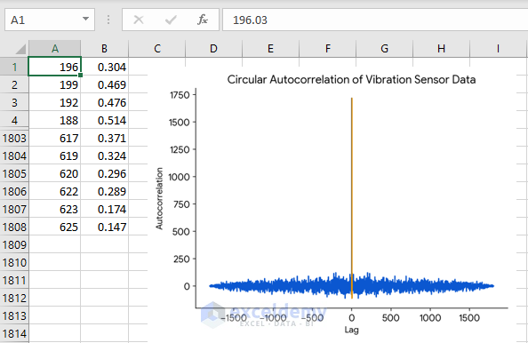
Thank you for sharing your experience with us. I understand you want to know how the lag segments work to properly configure your digitized vibration sensor data from rotating machinery.
Here are factors to consider:
1. Longer data means you can use more lag values without losing reliability.
2. More frequent data collection might need more lag values to find detailed patterns.
3. If you expect specific patterns, use enough lag values to catch them.
4. To detect repeating patterns, use enough lags to cover potential periods.
5. More lags require more calculations, potentially slowing processing. Balance accuracy and efficiency based on available resources.
6. With your data resolution, you could start with around 40-50 lags to capture potential patterns within a rotation.
7. Finally, there’s no universally optimal lag length. It depends on your data, analysis objectives, and computational constraints.
Let’s calculate the autocorrelation with a data range similar to yours using a different technique. Since you have significantly large data, you can consider this method. I am going to calculate autocorrelation using Excel VBA to make the process faster and more accurate. Follow the steps:
1. Line up your data.
2. Run the below VBA code:
As a result, you will obtain the scatter chart visualizing your output.
You can use the effective methods mentioned in the article too. Hope this helps!
Regards,
Yousuf Khan Shovon
Hello G,
Thank you for sharing your experience with us! I understand you are facing time issues with your attendance & overtime calculations. You mentioned that you could only get AM time but not PM. This is interesting because Excel has no built-in time format that shows only AM and not PM. All standard time formats like h:mm AM/PM, hh:mm AM/PM, and m:ss AM/PM display both AM and PM for times before and after noon, respectively.
The reason you are facing this issue could be your regional settings might be set to a locale that uses a 24-hour clock instead of a 12-hour clock with AM/PM indicators. To check your regional format and adjust your settings:
1. Go to Control Panel.
2. Click Clock and Region to see your existing time format.
Another reason could be a Custom Format has been applied to the cells that only show AM and hides PM. Whatever the reasons are, you can make it right using the specific time format. Follow the steps:
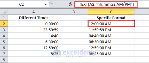
1. Select a blank cell where you want the output.
2. Enter the following TEXT formula and press Enter.
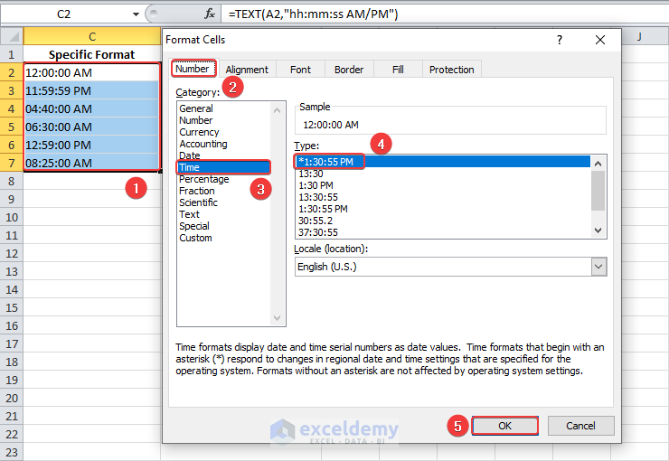
=TEXT(A2,"hh:mm:ss AM/PM")As a result, the TEXT function converts different time values into text strings. If you want to calculate these times later, then set a custom format:
1. Select the target cells and press Ctrl + 1.
2. In the Format Cells dialog, click Time under Category.
3. Select the desired format code in the Type box and click OK.
Thus, you embed the desired time formats.
Regards,
Yousuf Shovon
Hello Roge,
Thanks for your feedback! I understand you want to create a line chart race horizontally. Yes, it is possible to do so using Excel’s built-in animation features, VBA, or Flourish Studio. Though, I would recommend using Flourish Studio because it is so much easier.
To create a line chart race horizontally with Excel data and Flourish Studio, follow these steps:
1. Login into Flourish Studio.
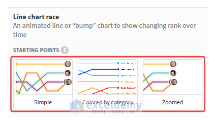
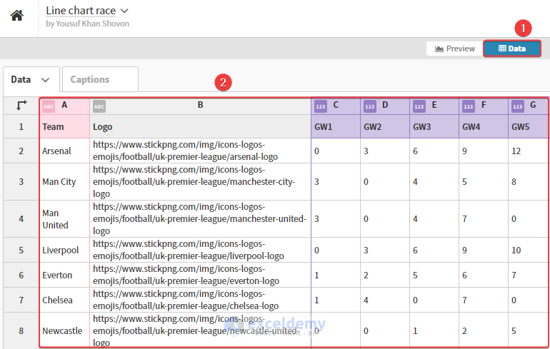
2. Create a new project. Scroll down and select any template.
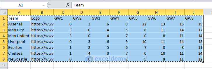
3. Line up your Excel data and copy.
4. Go to the site again. Click Data and feed your Excel data by pasting.
5. Now, you can preview your data and modify it according to your requirements.
6. Finally, click on Export & Publish.
If you still need to implement this in Excel, post your problem at our Exceldemy Forum with sample data. Our team will reach out to you as soon as possible.
Regards,
Yousuf Khan Shovon
Hello Ryan,
To filter the double letter bins out from this list without using a filter function, see if using a range of characters works instead. Then, [0-9] should only match numeric characters. Follow the below steps:
1. Open the Custom AutoFilter dialog. (Read the article if necessary)
2. Enter Bin in Filed and type the below condition in Criteria:
20??[0-9][!A-Z]AHere,
– 20?? matches the first four characters (2000 to 2099).
– [0-9] matches the fifth character that it’s a numeric digit and not a letter.
– [!A-Z] matches any character that is not a letter from A to Z, effectively excluding double letters in the fifth and sixth positions.
– A matches the final “A” in the bin code.
As a result, the filter criteria will accurately find bins in the 2000A range that have a single numeric digit followed by a single letter “A” at the end, excluding those with double letters like 200AA, 200BA, and 200CA.
Regards,
Yousuf Khan Shovon
Hello M E,
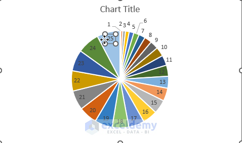
The above steps are the right ways to show leader lines in the Pie chart when not working. It worked perfectly for me when I manually dragged them but in your case, it did not work probably for these reasons:
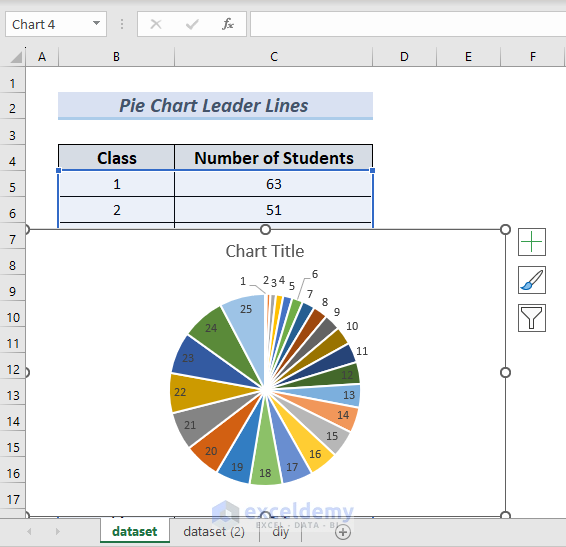
1. Best Fit is your selected option.
2. You are not dragging the labels in the correct way.
The leader lines in any chart will only appear if the labels are positioned with Best fit or manually dragged outside of the pie wedges if other options (like Outside End) are selected.
Even then the leader lines appear if the Best fit has to move the label position because they are further from the point they are labeling.
Solution 1:
Leader lines may not appear if Excel with the Best Fit option selected feels they are unimportant.
Excel uses the Best Fit option to arrange the labels without overlapping as best it can. If the Pie wedges are large enough, the labels go to the Inside End. Alternatively, they go to the Outside End to prevent overlaps, in which case the leader lines appear automatically.
Therefore, you sometimes have to manually drag them to appear.
Solution 2:
The correct way to drag (upon Show Leader Lines checked) is to double-click on a data label to select an individual data label. Then, drag the label further from its original point when you see the four headed arrow.
These steps will show you the leader lines in your Pie chart. Further, if you have any difficulties in this case, share your working file here or in our ExcelDemy Forum and we will go through it.
Regards,
Yousuf Khan Shovon
Hello Telkom University,
Thank you for sharing your concern here. The step-1 of this article ensures setting up the format and the integrity and accuracy of test cases of the testing process. However, I will list some additional approaches you can take to maintain the integrity and accuracy of test cases:
1. Worksheet Protection:
Approach: Protect worksheets with a password. Limit access permissions to authorized team members. Regularly review and update access rights based on the testing.
2. Data Validation:
Approach: Set up data validation rules in Excel. Specify allowed data types and values for each cell. This prevents errors caused by incorrect data entries during testing.
3. Cell Comments and Documentation:
Approach: Add comments to cells for additional information. Maintain a separate documentation sheet detailing test case specifics, ensuring clarity for team members.
4. Consistent Formatting:
Approach: Establish a consistent format for your Excel sheets. Use the same font styles, colors, and cell formatting throughout. Consistency enhances readability and reduces confusion.
5. Regular Reviews:
Approach: Schedule regular team reviews of the Excel sheets. Discuss any updates or changes to ensure everyone is aligned. Use this as an opportunity to address questions and concerns.
6. Backup:
Approach: Regularly back up your Excel sheets to a secure location. Cloud storage is a good option. This ensures data recovery in case of accidental changes.
7. Excel Features:
Approach: Use Excel features like Named ranges, filters, and Conditional Formatting. These tools help organize and highlight critical information, making test cases more accessible.
8. Training and Documentation:
Approach: Conduct training sessions on Excel usage and the established processes. Document guidelines for creating, updating, and maintaining test cases.
Take these steps to properly maintain the integrity and accuracy of the test cases throughout the testing process for a banking application.
Regards,
Yousuf Khan Shovon
Hello HUONGPT,
Thanks for sharing your experience with us!
The code shared in this article is designed to import data from a Google Sheets web version to an Excel offline version. It uses a Google Sheets key to access the data.
To modify this code for Microsoft 365 Excel online version, you would need to adapt it to use the appropriate URL for your Microsoft 365 Excel file. Microsoft 365 Excel doesn’t use a key like Google Sheets, but rather the URL of the shared document. Use the below VBA code instead:
You can also import data from online Excel without VBA quite easily. Here is how:
1. When you open your Online Excel file there is an option called Edit.
2. Select Edit in Online Excel >> then it will open in Desktop Excel.
3. Now, you will have all the options. It is as easy as it sounds!
Hope these suggestions help. Keep excelling.
Regards,
Yousuf Khan Shovon
Hello Smith,
Thanks for sharing your experience with us. The #ARG! error (Argument Error) in Excel generally occurs when a function or formula receives incorrect or invalid arguments. In the above code, I have noticed a few varibale name mismatches. Such as:
The function is defined as “Generate_QR” but it is assigned the name “GenerateQR” in the code. “My_Cell” should be “MyCell“. Also, The URL construction has double ampersands (“&&“) which are not needed.
As a result, the VBA script is returning these errors. Thanks for pointing out this to us. We greatly appreciate your feedback.
I have fixed the issues of the code. Try the below code instead:
Regards,
Yousuf Khan Shovon
Hello RYAN,
Thank you for sharing your experience.
I believe you want to auto-populate Word documents from multiple Excel data like a purchase form. The reason you were able to display only one item after following the above steps is that the Mailings feature merges through only one entity for each line.
However, it is possible to display every line of the Purchase form using 2 easy steps.
Let’s start creating the dataset as per your requirements:
Afterward, let’s create another dataset in Word and follow the steps 3 to 9 of this article. Thus, we get the first line data according to your dataset. Now, we can toggle through each line data using the toggle buttons.
Or, we can display the desired number of lines in a single Word file.
Go to Finish & Merge >> Edit Individual Documents.
Put the number of lines you want to populate >> OK.
As a result, you get all the lines of data in your Word file.
Regards,
Yousuf Khan Shovon
Thank you so much for the useful note, ASD. We have included it in the article for our users to understand that step better. Much appreciation from ExcelDemy. Keep sharing your experience with us.
Hello JOE,
Thank you for sharing your experience with us. Since you have no Bounds command in your Excel 2016 version, let’s find an alternative way. Today, I am going to show you how to zoom your charts using VBA applicable in any Excel version. Let’s dive into it.
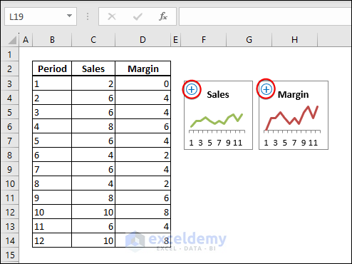
1. First, create (+) and (-) buttons in your workbook >> name them Zoom_Button in the NameBox. Or, you can copy them from the attached workbook and paste them into your chart.
2. Enter the below VBA code to your module >> Assign the Zoom_Chart macro in the buttons:
(If you do not understand this step, see this article)
How to Write VBA Code in Excel
The VBA code:
3. Click the Plus (+) button to zoom in on your chart.
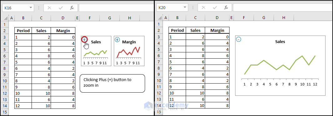
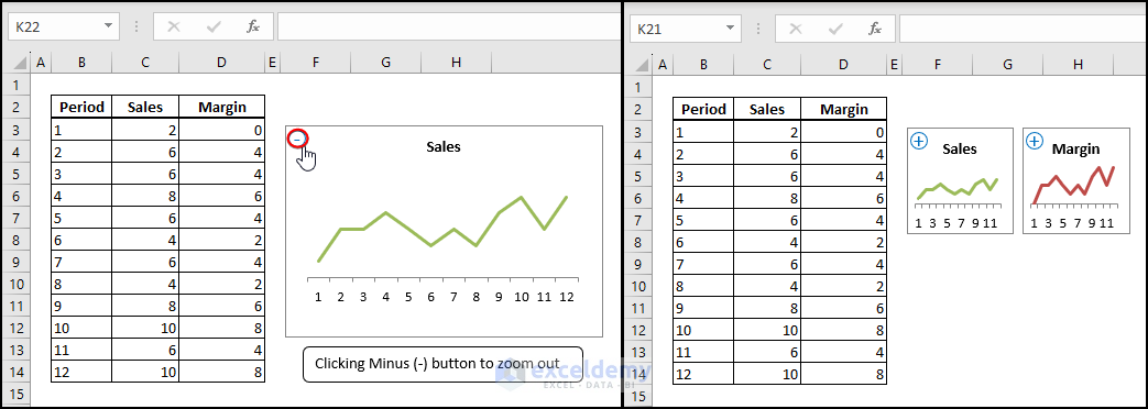
4. Click the Minus (-) button to zoom out on your chart.
You can set the zoom height and width in the given code in these lines:
Note: Here, 3 means 300% zoom and 2 means 200% zoom.
Download the workbook file here to practice.
Zoom Excel Chart.xlsm
Best Regards,
Yousuf Khan Shovon
Hello Mike,
Thank you for sharing your experience with us!
I understand you are getting non-clickable link text when you are copying the URL from web browsers. Also, the Paste Special command is not responding which would solve the issue in your case. Unfortunately, Paste Special command does not offer the Paste Link option while pasting web URLs.
But Excel directly inserts a hyperlink to a copied URL when you:
1. Copy the URL from a web browser >> select the cell where you want to paste >> paste the URL in the Formula Bar.
2. Alternatively, you can directly paste the URL to a cell >> go to Formula Bar >> press Enter.
This will convert the Text link to Hyperlink. You can also use the HYPERLINK function to get clickable URL links(read the article).
How to Use Excel HYPERLINK Function
Regards,
Yousuf Shovon
Hello MISLED READER,
Thank you for reading our article and your feedback. You have specified an incorrect use of the IPMT function that does not consider the start and end dates. And, you are correct about the fact that the method calculates the interest payable in the 1st period of a 5 year note represented by the hardcoded “1” used in the “PER” section of the formula. The IPMT function returns interest rates based on periods and not specific calendar dates. Thank you for pointing out the article gap to us. We will fix the issue with correct information. For now, we will show you another method here.
You can use the other Excel basic formula to calculate the interest between two dates. Or, enter a custom VBA function as described below.
This function will take the loan details, including start and end dates, as input arguments and return the interest amount.
Here is the syntax and arguments of the CalculateInterest function I have created:
Here are the steps to implement the function:
1. Save the below VBA code to a Module.
2. Now, enter the VBA function in cell C11 >> press Enter key to get the interest.
This formula calculates the interest between February 22, 2022, and March 24, 2022, based on the provided loan details.
Feel free to let us know your future queries and suggestions as we always appreciate them. Thank you.
Regards,
Yousuf Shovon
Hello Anthony,
Please, see the forum post to ignore cells when applying the SORT function.
Ignoring Null Cells In The Sort Function
Regards,
Yousuf Shovon
Hello Neil,
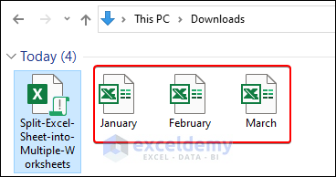
Yes, there is a way to name the resultant files using Excel VBA. I am modifying the VBA code to split the column into multiple workbooks given above. This code will rename the new files as month names using monthNames () array.
Here is the modified code:
Steps:
1. Enter the code in a module >> close the Visual Basic window.
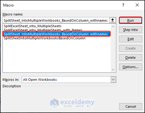
2. Go to the sheet you want to split >> Click on Developer >> Macros.
3. In Macro dialog, select SplitSheet_IntoMultipleWorkbooks_BasedOnColumn_withnames >> Run.
4. Consequently, the new files appear with declared names.
Note: The new files are created in .xls format as you requested. You can change the format in the code if you want.
I hope this was helpful to you. Let me know if you have any further queries.
Best Regards,
Yousuf Shovon
Dear Mike,
I understand you wish to insert a range to have the text as input. Here is the modified code to do so.
Also, you can insert a data range by adding variables. To know more about this, see this comment.
Hello PENELOPE JORDAN,
We are glad these methods were helpful to you. Though it seems, you are facing issues with the INDEX & MATCH method for multiple columns. If you are talking about the #NA! error using the given formula, it can be solved with an easy step. Just fill up the Product column with the proper value first and enter the given formula afterward. Thus, you will obtain the desired result.
Try this way and let us know if it works.
Regards,
Yousuf Khan Shovon
Hello JACK MACEY,
I understand you are facing issues while creating the weekly and monthly sheets using the same given code. The provided code works perfectly for Daily frequency. But for Weekly and Monthly intervals, you have to adjust the parameter of the frequencies in the code accordingly.
In this line below, we have declared the parameter of the frequency.
We have to add the interval=1wk or interval=1mo parameters to the URL, which specify the Weekly and Monthly intervals.
Here are the modified codes.
For Weekly frequency,
And for Monthly frequency,
Try this way. And, let me know if it works.
Regards,
Yousuf Khan Shovon
Thank you for your very useful suggestion, VAIBHAV SRIVASTAVA. I understand you suggested summing a text string which is much more relatable to this article. And to do so, you can merge the SUM, VALUE, and TEXTSPLIT functions. Here is the combined formula:
=SUM(VALUE(TEXTSPLIT(A1,"+")))Don’t hesitate if you have further suggestions for us. Thanks again.
Regards,
Yousuf Khan Shovon
Dear COLM,
Thank you for your very useful suggestion. I am including the note in the article with much appreciation.
Regards,
Yousuf Khan.
Hello NISHANTH VJ,
Thank you for your concern. Though I am afraid I am having trouble understanding the query clearly. Assuming you wish to modify the formula to account for the cost even in different forms every time you check in, you can use the weighted average cost of goods sold (COGS) method. This method calculates the average cost of all goods sold during a period, taking into account the varying costs of different ingredients.
The formula:
Food Cost Percentage = (Total Cost of Goods Sold ÷ Total Revenue) x 100To calculate the total cost of goods sold, you can use the following formula:
Total Cost of Goods Sold = (Beginning Inventory + Purchases - Ending Inventory) x Weighted Average Cost per UnitTo calculate the weighted average cost per unit, you can use the following formula:
Weighted Average Cost per Unit = Total Cost of Goods Available for Sale ÷ Total Units Available for SaleBy using this modified formula, you can account for the fluctuations in the cost of food and beverage and calculate your food cost percentage accurately, even if the cost of ingredients varies over time.
Regards,
Yousuf Khan Shovon
Dear RICH SAUNDERS,
I understand your frustration with trying to find specific INDEX/MATCH assistance for your Excel project. Here, I’ll create the Summary tab using INDEX/MATCH functions to connect the other four tabs.
To begin, let’s assume that your four tabs are named Dataset1, Dataset2, Dataset3, and Summary. To retrieve data from the Dataset1 tab, use the following formula:
=INDEX(Dataset1!$A$1:$O$40,MATCH($A2,Dataset1!$A$1:$A$40,0),MATCH(B$1,Dataset1!$A$1:$O$1,0))Note: Be sure to update the tab name and range of cells to match the appropriate tab and data range.
I hope this helps! Let me know if you have any further questions.
Regards,
Yousuf Khan Shovon
Hello FRANK,
Glad to know the basic methods were useful to you. We further appreciate your valuable insights in addition to these methods. We will look into the advanced techniques and add them in the future. Thank you.
Regards,
Yousuf Khan
Hello ARCHIE,
I understand you wish to fix the #VALUE! error for VLOOKUP. In your case, the reason this is returning #VALUE! error for alpha-numeric values is that it is trying to convert the text values to numbers using the VALUE function. The VALUE function is designed to convert text that represents a number to an actual number. When it encounters alpha-numeric values, it cannot convert them to numbers, hence the error.
Fortunately, you can fix this by modifying the formula by replacing the VALUE function with the TEXT function. The TEXT function converts a value to text in a specific number format. Try the modified formula given below:
=IF(ISNA(VLOOKUP(TEXT($A42,"0"),PROJECT_LIST!$A:$C,3,FALSE)),"",VLOOKUP(TEXT($A42,"0"),PROJECT_LIST!$A:$C,3,FALSE)&" ")Let me know with a demo dataset if you still face issues. Good luck!
Note: Make sure data are sorted in ascending to descending order in the lookup table.
Regards,
Yousuf Khan
Hello MONTY,
Thank you so much for your useful suggestion. Our Exceldemy team will include the note in the article as soon as possible. We always appreciate any further concerns or suggestions you may have.
Hello ADITYA,
You’re welcome! We are glad to hear that you found the solution to your issue. Unprotecting the workbook can indeed resolve the issue of being unable to set the visible property of the Worksheet class. It’s great to see that your dynamic VBA code is working as expected. Let us know if there’s anything else we can help with.
Regards,
Yousuf Khan
Hi MICHAEL,
The errors you’ve mentioned could indicate that the workbook is either very hidden or corrupted. There are two levels of worksheet hiding: hidden and very hidden. From a user’s perspective, the difference is that a very hidden sheet cannot be made visible through the Excel user interface, and the only way to unhide it is with VBA.
Since you’ve used VBA to work with the worksheets and they still appear hidden, you can try a different VBA code to check if they’re very hidden and unhide them. Here’s the VBA code to unhide all very hidden sheets:
Note: This code only works for very hidden sheets, not worksheets that are hidden normally. If you want to display all hidden sheets, use the code below.
Give it a try and let me know if it works.
Best Regards,
Yousuf Khan