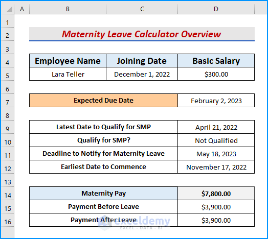
This is an overview of the maternity leave calculator. It calculates Statutory Maternity Pay (SMP) and Statutory Maternity Leave (SML).
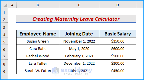
Step 1 – Create a Dataset
- Enter Employee Name, Joining Date, and Basic Salary in columns B, C, and D.
- Enter data.
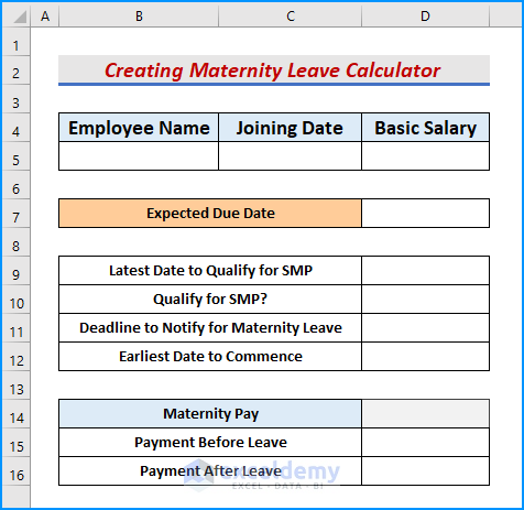
Open a new sheet and add the following headers:
- Expected Due Date: date of birth.
- Latest Date to Qualify for SMP: apply the Statutory Maternity Pay by adding 41 weeks before the child’s birth.
- Qualify for SMP?: To qualify for the additional SMP, the employee must have a minimum 1-year service.
- Deadline to Notify for Maternity Leave: 15 weeks before the child’s birth.
- Earliest Date to Commence: 11 weeks before maternity leave.
- Maternity Pay: Total maternity payment based on the basic salary.
- Payment Before Leave: Half the total payment.
- Payment After Leave: Half the total payment.
Read More: How to Create Leave Tracker in Excel
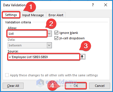
Step 2 – Utilize the Data Validation Feature to Import Data from a Table Array
- Select B5 and go to the Data tab → Data Validation in Data Tools.
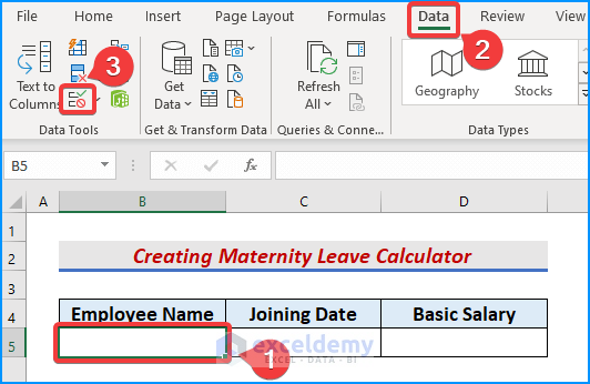
- Select Settings → Choose List in Allow → in Source, select the table used in Step 1.
- Click OK.
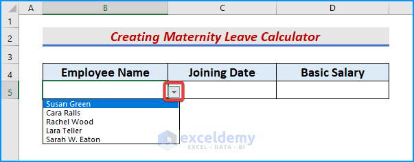
- Click the Dropdown icon in B4 to see the employee list.
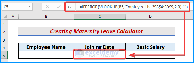
Step 3 – Merge the VLOOKUP and the IFERROR Functions to Display Data
- Enter the following formula in C5,
=IFERROR(VLOOKUP(B5,'Employee List'!$B$4:$D$9,2,0),"")- Press Enter or Tab.
- Enter the following formula in D5,
=IFERROR(VLOOKUP(B5,'Employee List'!$B$4:$D$9,3,0),"")- Press Enter.

Formula Breakdown:
- VLOOKUP(B5,’Employee List’!$B$4:$D$9,3,0) looks for the 3rd row of the data in B5 in B4:D9.
- IFERROR(VLOOKUP(B5, ‘Employee List’!$B$4:$D$9,3,0),””) It returns a blank cell if there’s missing data or an error.
Read More: How to Create Employee Monthly Leave Record Format in Excel
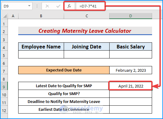
Step 4 – Combine the IF Function and Excel Formulas to Set the SMP Conditions
- Enter the formulas and press Enter or Tab:
- In D9:
=D7-7*41subtracts 41 weeks from the Expected Date in D7.
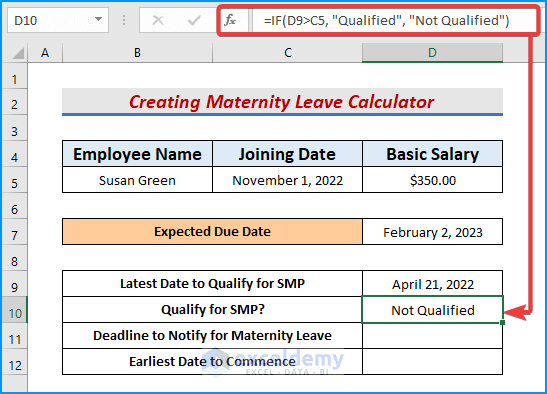
- In D10:
=IF(D9>C5, "Qualified", "Not Qualified")determines if the condition is True or False and returns Qualified or Not Qualified.
- In D11:
=D7+7*15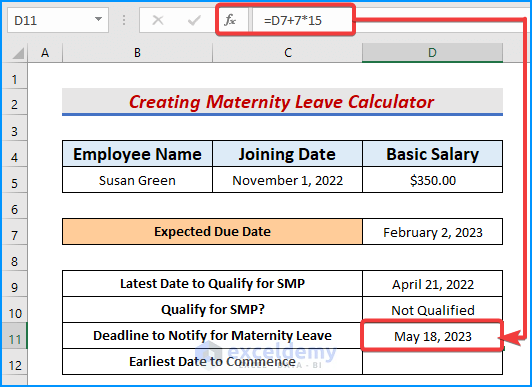
- In D12:
=D7-7*11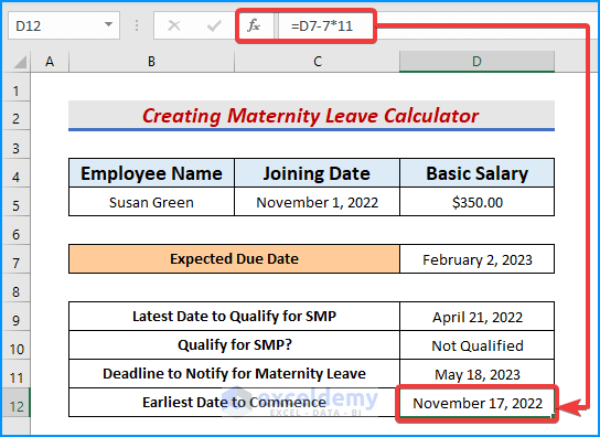
Read More: How to Track Employee Vacation Time in Excel
Step 5 – Merge the IF and the IFERROR Functions to Calculate the Maternity Pay
- Enter the following formulas and press Enter.
- In D14:
=IFERROR(IF(D10="Qualified",D5*52, D5*26),"")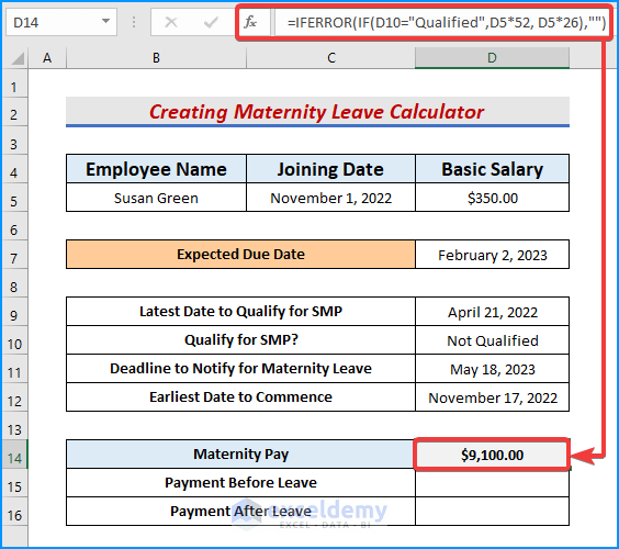
- In D15:
=IFERROR(D14/2,"")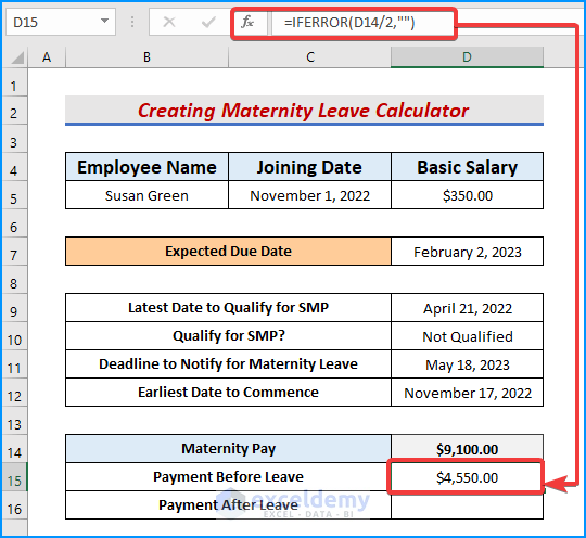
- In D16:
=IFERROR(D14/2,"")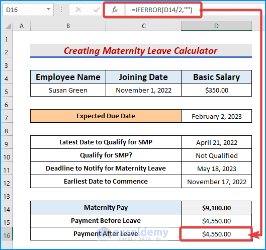
Formula Breakdown
- IF(D10=”Qualified”, D5*52, D5*26) multiplies 52 by the Basic Salary if the employee is Qualified. Otherwise, by 26.
- IFERROR(IF(D10=”Qualified”, D5*52, D5*26),””) returns blank cells if the reference cells are blank.
Read More: How to Create Employee Leave Record Format in Excel
Step 6 – Track Maternity Timeline and Analyze the Maternity Leave Calculator
- Enter the due date in D7.
- Go to B5 and select the employee.
- Observe the GIF.
Download Practice Workbook
Download the workbook and practice.
<< Go Back to Excel Employee Leave Tracker | Excel HR Templates | Excel Templates
Get FREE Advanced Excel Exercises with Solutions!
