We’ll use a dataset of 5 employees of a company to create a leave tracker.
![]()
Step 1 – Create a Summary Layout
- Create a Summary sheet.
- Select cell F1.
- From the Insert tab, select the drop-down arrow for Illustrations.
- Choose Picture and select This Device.
![]()
- A dialog box called Insert Picture will appear.
- Select your company logo and click Insert.
![]()
- We are inserting our website logo to show the process.
![]()
- Select the range of cells B4:I4 and select the Merge & Center option from the Alignment group.
- Insert the title. We set the file title as Employee Leave Tracker. Keep your desired formatting to the cell.
![]()
- In cell B6, write the title Year.
- In cell C6, insert the current year.
![]()
- In the range of cells K8:L14, specify the leave types and their short codes. We put 6 different types of leaves.
![]()
- Select cell B8:I8.
- Select the Merge & Center option and write down the table title. We put it as Year Summary.
![]()
- In cell B9, write the column name as Employee Name and set the range of cells B10:B14 for 5 employees.
![]()
- In the range of cells C9:H9, denote the leave short forms.
![]()
- Set 2 Total cells, one for the column and the other for the rows.
![]()
- Here’s our summary layout.
![]()
Read More: How to Track Employee Vacation Time in Excel
Step 2 – Build Tracker List for Each Month
- Create a new sheet and rename it as Jan.
- In the Home tab, select the Format option from the Cells group and click on Column Width.
![]()
- A small dialog box called Column Width will appear.
- Set the column width to 2.50 and click OK.
![]()
- Select cell AF1 and insert your company logo similarly as in Step 1.
![]()
- In cell B4, insert the following formula:
="January"&Summary!C6
- Press Enter to store the data.
![]()
- As the month of January has 31 days, select 32 columns that are from B6:AG6. Select the Merge & Center option from the Alignment group.
- In the merged cell, insert the following formula and press the Enter key.
=B4
![]()
- Name cell B7 as Days and cell B8 as Employee Name.
![]()
- Modify the cell format for the range of cells B9:B13 and keep them to input the employee names.
![]()
- Use the DATE function to get the date in cell C8:
=DATE(Summary!$C$6,1,1)
![]()
- In cell D8, insert the following formula and drag the Fill Handle icon to the right to copy the formula until you get 28.
=C8+1![]()
- For the last 3 cells AE8:AG8, insert the formula shown below:
=IF(MONTH($AD8+1)>MONTH($C$8),"",$AD8+1)
Breakdown of the Formula
- MONTH($AD8+1): This function returns 1.
- MONTH($C$8): This function returns 1.
- IF(MONTH($AD8+1)>MONTH($C$8),””,$AD8+1): This function returns the date.
![]()
- In cell C7, insert the following formula:
=IF(C8="","",INDEX({"Su";"M";"Tu";"W";"Th";"F";"Sa"},WEEKDAY(C8,1)))Breakdown of the Formula
- WEEKDAY(C8,1): This function returns 7.
- INDEX({“Su”;”M”;”Tu”;”W”;”Th”;”F”;”Sa”},WEEKDAY(C8,1)): This function returns Sa.
- IF(C8=””,””,INDEX({“Su”;”M”;”Tu”;”W”;”Th”;”F”;”Sa”},WEEKDAY(C8,1))): This function returns the day name Sa.
![]()
- Drag the Fill Handle icon to the right to copy the formula up to cell AG7.
![]()
- Select cell C9.
- In the Data tab, select the drop-down arrow of the Data Validation option from the Data Tools group.
- Select the Data Validation option.
![]()
- A small dialog box called Data Validation will appear.
- In the Setting tab, select the drop-down arrow below the Allow title and choose the List option.
- Insert the cell reference $AH$8:$AM$8 in the box below Source or simply select the range with your mouse.
- Click OK.
![]()
- You will see a drop-down arrow that contains all the short forms.
- Drag the Fill Handle icon in the range of cells C9:AG13 to copy the drop-down arrow in all the cells.
- Mark the weekends with a different color so that you can easily find them.
![]()
- Select the range of cells AH6:AM6 and choose the Merge & Center option.
- Name the merged cell as Total.
![]()
- Use the COUNTIF function in the following formula in cell AH9:
=COUNTIF($C9:$AG9,AH$8)+0.5*COUNTIF($C9:$AG9,AH$8&"H")+0.5*COUNTIF($C9:$AG9,"H"&AH$8)
Breakdown of the Formula
- COUNTIF($C9:$AG9,AH$8): This function returns 1.
- COUNTIF($C9:$AG9,AH$8&”H”): This function returns 0.
- COUNTIF($C9:$AG9,”H”&AH$8): This function returns 0.
- COUNTIF($C9:$AG9,AH$8)+0.5*COUNTIF($C9:$AG9,AH$8&”H”)+0.5*COUNTIF($C9:$AG9, “H”&AH$8): This function returns the day name 1.
![]()
- Drag the Fill Handle icon to the range of cells AH9:AM13.
![]()
- In the range of cells AH8:AM8, insert the following formula to show the leave type short forms.
=Summary!C9
![]()
- In cell AH7, use the SUM function:
=SUM(AH9:AH13)
![]()
- Drag the Fill Handle icon to copy the formula up to cell AM7.
- The leave tracker for the month of January will be ready to use.
![]()
- Create the monthly leave tracker sheets for the other months of the year. You can copy most of the content and change the month.
![]()
Read More: How to Create Employee Monthly Leave Record Format in Excel
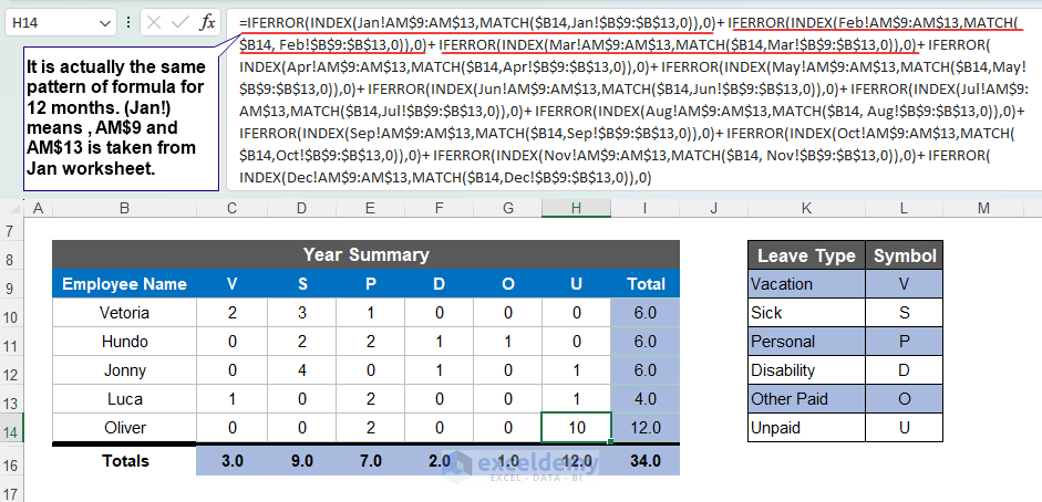
Step 3 – Generate the Final Leave Tracker
- Insert the following formula into cell C9.
=IFERROR(INDEX(Jan!AH$9:AH$13,MATCH($B10,Jan!$B$9:$B$13,0)),0)+IFERROR(INDEX(Feb!AH$9:AH$13,MATCH($B10,Feb!$B$9:$B$13,0)),0)+IFERROR(INDEX(Mar!AH$9:AH$13,MATCH($B10,Mar!$B$9:$B$13,0)),0)+IFERROR(INDEX(Apr!AH$9:AH$13,MATCH($B10,Apr!$B$9:$B$13,0)),0)+IFERROR(INDEX(May!AH$9:AH$13,MATCH($B10,May!$B$9:$B$13,0)),0)+IFERROR(INDEX(Jun!AH$9:AH$13,MATCH($B10,Jun!$B$9:$B$13,0)),0)+IFERROR(INDEX(Jul!AH$9:AH$13,MATCH($B10,Jul!$B$9:$B$13,0)),0)+IFERROR(INDEX(Aug!AH$9:AH$13,MATCH($B10,Aug!$B$9:$B$13,0)),0)+IFERROR(INDEX(Sep!AH$9:AH$13,MATCH($B10,Sep!$B$9:$B$13,0)),0)+IFERROR(INDEX(Oct!AH$9:AH$13,MATCH($B10,Oct!$B$9:$B$13,0)),0)+IFERROR(INDEX(Nov!AH$9:AH$13,MATCH($B10,Nov!$B$9:$B$13,0)),0)+IFERROR(INDEX(Dec!AH$9:AH$13,MATCH($B10,Dec!$B$9:$B$13,0)),0)Breakdown of the Formula
- MATCH($B10,Jan!$B$9:$B$13,0): This function returns 2.
- INDEX(Jan!AH$9:AH$13,MATCH($B10,Jan!$B$9:$B$13,0)): This function returns 0.
- IFERROR(INDEX(Jan!AH$9:AH$13,MATCH($B10,Jan!$B$9:$B$13,0)),0): This function returns 1.
![]()
- Copy the formula up to cell H14 by dragging the Fill Handle icon.
![]()
- In cell I10, use the SUM function to sum the range of cells C10:H10:
=SUM(C10:H10)
![]()
- Double-click on the Fill Handle icon to copy the formula up to cell I14.
![]()
- In cell C16, insert the following formula:
=SUM(C10:C14)
![]()
- Copy the formula up to cell I16 using the Fill Handle icon.
![]()
- The leave tracker is completed and ready to use.
![]()
Read More: How to Create Employee Leave Record Format in Excel
Step 4 – Verify the Leave Tracker with Data
- Input employee names in the range of cells B10:B14.
- Input some data for January in the sheet Jan.
![]()
- Input some values for the months of February in sheets Feb.
![]()
- If you check the Year Summary table, you will find our formula is extracting the values from the month sheets and showing us individual employees and individual leave types.
![]()
Read More: How to Create Maternity Leave Calculator in Excel
<< Go Back to Excel Employee Leave Tracker | Excel HR Templates | Excel Templates
Get FREE Advanced Excel Exercises with Solutions!

Hi! Am Babalola Olona. I want to say a very big thank you to ExcelDemy for this great article as this will go a long way to help build up a lot of learners.
While I am happy that am able to learn a lot from this piece I however have challenges comprehending Step 3 “Generate Final Leave Tracker”, I really cant understand the formula used “IFERROR, INDEX, MATCH & SUM”.
I can’t also understand the rational behind the use of 0.5, “H” & in the COUNTIF function. i will be eternally grateful this FUNCTIONS can be further broken down for a better understanding.
Thank you.
Thanks a lot BABALOLA for the appreciation. It means a lot.
In response to your first question, let me break down the whole formula with IFERROR, INDEX, MATCH & SUM and explain it to you.
The first part of the formula here is IFERROR(INDEX(Jan!AH$9:AH$13,MATCH($B10,Jan!$B$9:$B$13,0)),0)
First of all the MATCH function looks through the value in range B9:B13 of Jan sheet whether it matches the value in cell B10. If it gets matched, it will return the related value according to the index from the AH9:AH13 range. The IFERROR Function is used to return a value(i.e. 0) if it can not find any proper value to return.
Similarly, I have gone through all 12 months’ sheets and added them with the SUM function.
In response to your second question, the & sign is used to concatenate cell AH$8 with the letter H. As it is considered a half match, 0.5 is multiplied. We have considered two half-matches to have the full match count.
Hello, I track leave for my company and need more rows than 5 (much more than 5 people), how do I insert rows without messing up the formula?
Dear Karlyn Martinez,
For your convenience, I have showed the task with following steps.
Steps:
● First, you have to recognize the pattern in the formula
● You can use Format Painter or drag the row to add a new row or rows for editing new data.
● Now add new data.
● Inset new rows in the Summary sheet.
● Insert the Entire row.
● Edit the code according to the main dataset. As now in Jan worksheet, new data is added, and so the range will be changed to AH$15 and $B$15.
Hope, this will be helpful for you.
Regards,
Joyanta Mitra
Excel & VBA Content Developer
We ran into issues with the large formula since our line number weren’t exactly like yours. For instance, I have 10 employees vs 7. We’re still working on it but not quite there yet. Wish there was an easier way to get the summary.
How do you record half day leave?
Hi KOH,
Thanks for reaching out to us! Unfortunately, the method discussed above doesn’t currently support recording half-day leave. We understand how frustrating that can be, and we’re sorry for any inconvenience caused. Rest assured, we’ll definitely work on overcoming this limitation in the future.
We’re grateful for your support of Exceldemy and we hope to make your experience even better in the future.
Best regards,
Aniruddah
Team Exceldemy
Hello – this tutorial has been so helpful – THANK YOU! I am however struggling to get my summary to pick up leave noted throughout the year when i carry out my test (as you do in your video)……I cannot work out where I have made an error as I thought I was being very careful to follow all of your instructions….can you please provide any help?
Hello Tracey
Thanks for your nice words. Your appreciation means a lot to us.
Creating a Leave Tracker in Excel requires multiple steps, so you may often get unintentional errors when following these steps. Do not worry! You can share your problem within the ExcelDemy Forum by attaching your workbook.
Regards
ExcelDemy
Hello
I am not having any luck with step 3 generate final leave tracker on the summary page. I have tried it many different ways with no luck. Can I send it to get some help?
Hello Bonnie
Thanks for reaching out. Though a few steps are needed, making mistakes along the way is obvious. But no worries! The ExcelDemy Forum is there to help. Just share your workbook and ask for advice.
Regards
Lutfor Rahman Shimanto
ExcelDemy
I have 100 employees. I made it but the summary doesn’t work!!
Dear Sanjeev
Thanks for visiting our blog and sharing your problem. After adding the desired rows, you must drag the Fill Handle icon to copy the existing formulas for new employees. We have improved the file and made the necessary formula adjustments based on your goal.
SOLUTION Overview:
You can download the solution file: https://www.exceldemy.com/wp-content/uploads/2024/05/Sanjeev-Fernandes-SOLVED.xlsx
Regards
Lutfor Rahman Shimanto
ExcelDemy
Great work guys!!! Your patience and responses
Hello Babajide,
Thanks! We are glad to hear that you found it great. We try our best to provide excellent services. Keep learning Excel with ExcelDemy!
Regards
ExcelDemy
Hi! I have a question regarding the Countif formula because I want to input 0.5 which is a half-day leave and have it reflect as 0.5 in the summary.
Hello HR,
If you want to input 0.5 as half day leave. You can use the following formula for Half Day (HD) column: =SUMPRODUCT(–($D9:$AH9=”HD”)*0.5)
It will look for all occurrences of “HD” within the range $D9:$AH9. Each “HD” will be counted as 0.5.
You will need to format the cells with 2 decimal places to properly show the decimal number otherwise it will show you rounded 1.
Regards
ExcelDemy
Hi
This is working brilliantly thank you. My only issue is when we add new employees onto the summary (we have over 150) they need sorting A-Z, however, whilst the employee names sort on the month views, the leave that has previously been entered for those employees does not move, meaning it is then listed against the incorrect employee. Is there any way around this please?
Hello AM,
Thanks for your appreciation. To keep leave data aligned with the correct employee after sorting, refer the names from the Month sheet into the summary sheet. This way, the data stays tied to each employee regardless of sorting changes.
Alternatively, consider using Excel’s INDEX-MATCH or XLOOKUP functions to pull data dynamically based on employee IDs, which would adjust automatically if names are resorted.
Regards
ExcelDemy
This has been really insightful. I appreciate it. Any idea on how we can colour code the Leave types? eg: having HD, S P, D, O ,U have different background colours. Also, is there a way to pre-input public holidays? i.e. like having a list of public holidays already in the Calendar so that people don’t bother choosing those dates for their leave. Lastly, how about if we want to avoid specific staff going on leave at the same time. eg. We only want one of Victoria, Ondo or Clark to go on leave at a time but not at the same time. I have managed to ask three different
Hello Mabel,
Thank you for your questions!
Color coding leave types: You can use conditional formatting in Excel. Create rules based on leave type values (e.g., HD, SP, etc.) and assign different colors to each.
Pre-inputting public holidays: List the public holidays in a separate range and use data validation to restrict leave selections to avoid those dates.
Preventing overlapping leave: You can use formulas like COUNTIFS to track the leave dates for specific employees and highlight conflicts.
Regards
ExcelDemy
I have learnt beautifully on here.
Please, I need a query that prompts me when specific employees are going on leave at the same time eg: Victoria, Hundo, Jonny are al going on leave at the same time.
Also, is it possible to have all public holidays already set on all the months for the year? if possible, kindly give an example of how to go about this please using the already created data set on here.
Thank you and well done with the amazing work you have been putting out.
Hello Mabel,
Thank you for your kind feedback! It means a lot to us.
Query for Overlapping Leaves: Add a helper column to concatenate names and leave dates using =A2&B2 (assuming Column A has names and Column B has leave dates).
Use COUNTIFS to identify overlaps:
=COUNTIFS(A:A, “Victoria”, B:B, B2) + COUNTIFS(A:A, “Hundo”, B:B, B2) + COUNTIFS(A:A, “Jonny”, B:B, B2)
Highlight rows where the result >1.
Public Holidays: Create a table for public holidays and link it using VLOOKUP or conditional formatting to flag dates in your tracker.
Example formula:
=IF(ISNUMBER(MATCH(B2, PublicHolidayRange, 0)), “Public Holiday”, “”)
Regards
ExcelDemy
I have created 2025 and now need to add 2 new employees. How do I do this?
Hello NancyP,
To add new employees to your leave tracker,
1. Simply insert rows for the new employees and input their relevant data, such as names, leave balances, and other details.
2. Then you need to adjust any formulas (such as leave accrual calculations) to accommodate the new rows. Include the newly added rows cell reference in the formulas.
3. Ensure that any drop-down lists or data validation rules are updated as well to include the new employee names.
Regards
ExcelDemy
This isn’t helpful as I’m new to Excel. I used the tutorial to show me how to create the tracker. I need to add 2 new employees to the tracker for 2025.
Is there a similar tutorial to show me how to do that?
Hello Nancy Poelvoorde,
To add new employees to your 2025 leave tracker, you can follow a step-by-step guide similar to creating the original tracker. Unfortunately, we don’t have an exact tutorial for your case, but you can adapt the existing guide by inserting rows for new employees and updating formulas or validation.
Existing Youtube Tutorial: How to Create Leave Tracker in Excel
Here, I have shown the step of adding new employee to the leave tracker. Add New Employee in the Leave Tracker
Regards
ExcelDemy
Hi, I have created the leave tracker following the video shared on youtube, i have been stuck on the second last part where you created a formula to repeat on each and every month, can you help me?
Hello Aluwani,
It sounds like you’re trying to apply a formula across multiple months in your leave tracker. Typically, you’ll need to use relative referencing or a dynamic formula to repeat the calculations. You can either copy the formula manually or use Excel’s drag-and-fill feature for cells with similar data patterns.
To directly copy the formula you can download the Excel File: Create-Leave-Tracker-2025.xlsx
For further help, check out the detailed guide in the video or feel free to provide more specifics about where you’re stuck!
Regards
ExcelDemy
Hi, My info for about 132 employees is not totalling properly. i read all comments and altered the formulas to match info but still it isnt giving me the total in the summary. please help
Hello Tay Tionne,
It sounds like there might be an issue with the formula references or data range in your summary section.
Double-check that the formula correctly includes all 132 employees and isn’t missing any rows. Also, ensure there are no blank cells or text entries in numeric columns, as they can cause calculation errors.
If possible, try using the SUM function with explicit ranges (e.g., =SUM(A2:A133)) to verify the totals.
Regards
ExcelDemy
Hi, I would love to add in a follow up date for each employee. Do you have a reference for that?
Hello Alyssa,
Yes, you can incorporate a follow-up date for each employee into your Excel leave tracker. Here’s how you can do it:
1. Add a ‘Follow-Up Date’ Column:
In your main tracking sheet (e.g., “Summary” or “Employee Leave Records”), insert a new column labeled “Follow-Up Date” next to each employee’s name.
Manually input the follow-up date for each employee as needed.
2. Automate Follow-Up Dates (Optional):
If you prefer to automate the follow-up dates based on certain criteria, such as a specific number of days after the last leave date, you can use Excel formulas. For example:
Assuming the last leave date is in column D, you can use the following formula in the “Follow-Up Date” column:
=IF(D2<>“”, D2 + 30, “”)
This formula adds 30 days to the last leave date. Adjust the number as per your requirements.
Regards
ExcelDemy
Hi thank you for the tutorial. I am at the end but when I try to copy over cells in the summary it brings up a file open box. Any feedback for where I have gone wrong?
Hello Va,
This usually happens when a formula is referencing an external workbook (for example, a cell or sheet that was copied from another file). When Excel can’t find that source, it prompts you with a File Open dialog.
Here’s what you can check:
1. Make sure all formulas in the Summary sheet refer only to sheets within the same workbook.
2. If you copied any formulas from another Excel file, re-enter them manually instead of pasting.
3. Check the formula bar for links like [WorkbookName.xlsx]SheetName! and remove those external references.
4. Also confirm that sheet names match exactly as shown in the tutorial.
Once all external links are removed, copying the cells should work without opening a file dialog.
Regards,
ExcelDemy