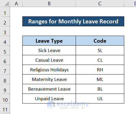
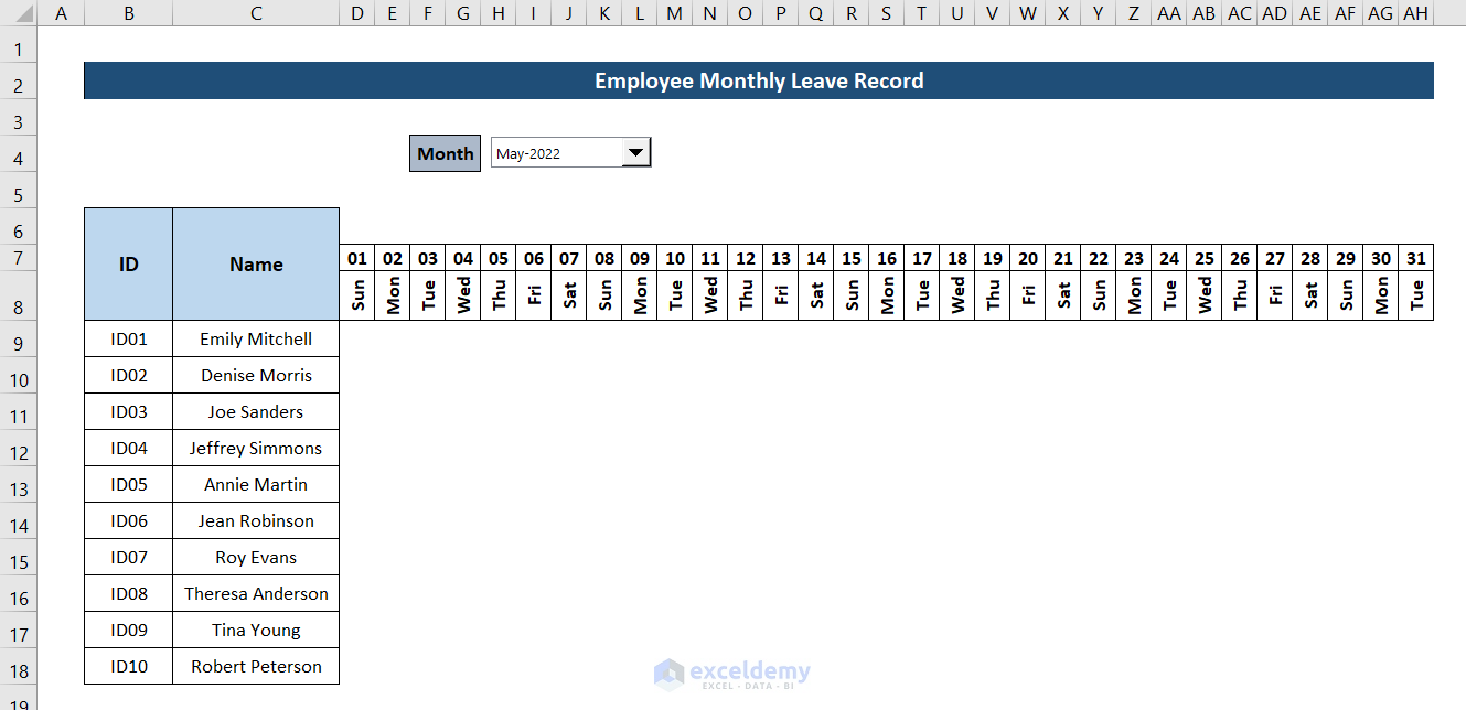
Step 1 – Make a List for All Types of Leaves
- Create a spreadsheet that contains all of the types of leaves the organization grants. Let’s assume, for our demo leave record format, there are a total of six types of leaves. We include that in this spreadsheet.
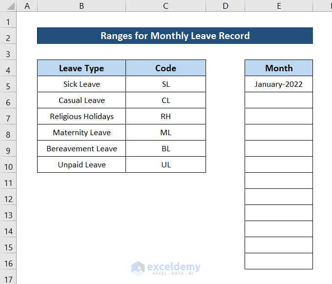
- Add a list of all the months. To enter months and years, let’s input them like this first.

- Select cell E4 and press Ctrl + 1 to format the cell.
- In the format cells box, go to the Numbers tab and select the Custom category on the left of the box.
- On the right side, type in mmmm-yyyy in the Type field.

- Click on OK. The date format will look something like this.
- AutoFill the column for the rest of the months.

- Make a list of all the employees and their IDs that will help us track their leaves.

Read More: How to Create Leave Tracker in Excel
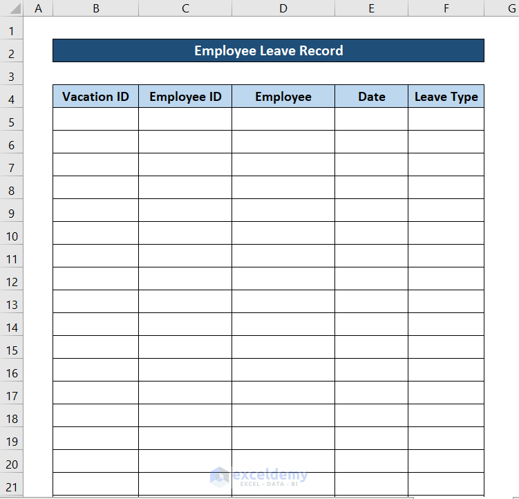
Step 2 – Create a Dataset to Record All Leaves Taken
- We have selected the following headings for the dataset.
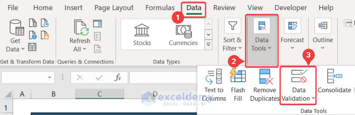
- We want to make a drop-down style input for the employees. Select the range from cell C5 to where you want to make the list and go to the Data tab.
- Select Data Validation from the Data Tools group.
- In the Data Validation box, select the Settings tab.
- In the Validation criteria section, select List in the Allow field, and in the Source field, manually select the IDs from the Lists spreadsheet or copy the following:
=Lists!$G$7:$G$16
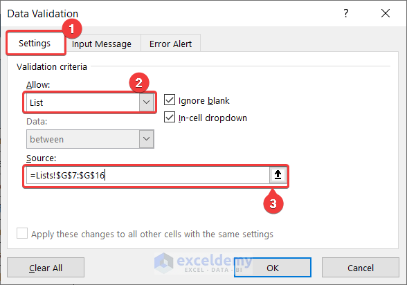
- Click on OK.
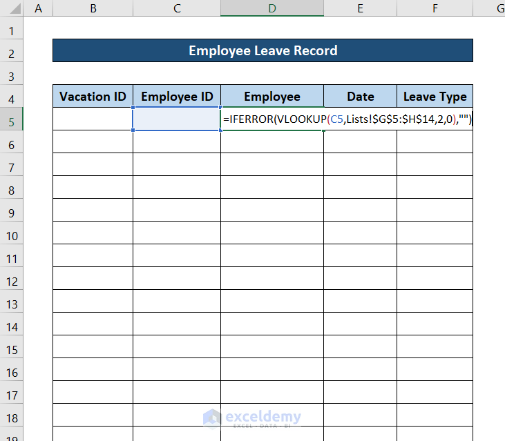
- Select cell D5 and copy the following formula:
=IFERROR(VLOOKUP(C5,Lists!$G$5:$H$14,2,0),"")
Breakdown of the Formula
IFERROR(VLOOKUP(C5,’Lists’!$B$9:$C$18,2,0),””)
VLOOKUP(C5,’Lists!$B$9:$C$18,2,0) looks for value in cell C5 in the range B9:C18 in the sheet called “Leave Calendar”. Argument “2” indicates the function will return a value from the second column, which is the short-code for leaves. And the final argument “0” indicates it has to be an exact match of cell C5.
The previous function is supposed to look for an exact match and return the value of the second column in the row it found the match. But there are cases where no match occurs. In case of that, we add the IFERROR portion of the formula. So that our charts’ cells won’t fill up with error warnings. The IFERROR(VLOOKUP(C5,’Lists!$B$9:$C$18,2,0),””) formula returns an empty string if the value doesn’t match the VLOOKUP function.
- Press Enter and replicate the formula for the rest of the cells in the column by double-clicking the Fill Handle on the bottom-right corner.
- Add a Data Validation field for cells in column F by repeating the process for cell F5.
- Similarly, select List in Allow field, and in the Source field, copy the following.
=Lists!$C$5:$C$10

- Click on OK.
- For Vacation IDs, select cell B5 and copy the following formula.
=C5&E5

- Press Enter.
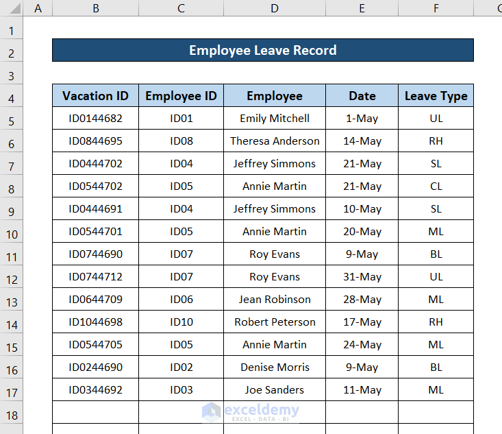
- Input some values in the dataset.
- Name the spreadsheet Leave Table.
Read More: How to Create Employee Leave Record Format in Excel
Step 3 – Create a Dynamic Monthly Leave Record Format
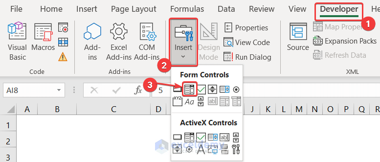
You might need to enable the Developer tab for this.
- Go to the Developer tab and click on Insert.
- Select Combo Box from Form Controls.
- Select a place by clicking and dragging on the spreadsheet.
- Right-click on the box and select Format Control from the context menu.

- Select the Control tab in the Format Control box.
- In the input range field, copy the following formula.
Lists!$E$5:$E$16
- Copy the following in the Cell link field.
$J$3
- In the Drop down lines field, write down 12 since we want all of the months to show in the list.

- Click on OK.
- Select the month in it and it will look something like this.

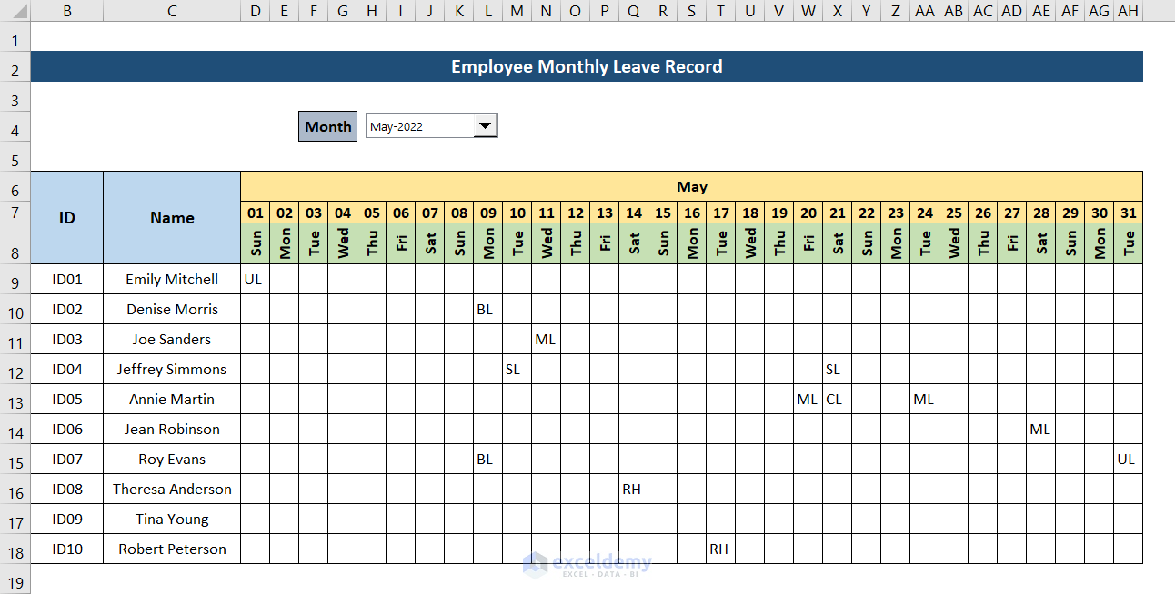
- Select cell Y4 and copy the following formula into it:
=INDEX(Lists!E5:E16,'Leave Calendar'!S4)
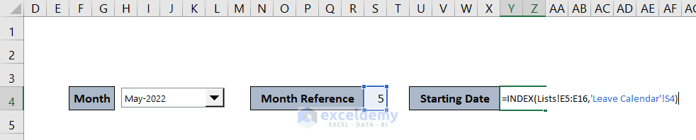
- Press Enter. These two cells will be helpful for future cell references.

- Put in the Employee IDs and Employee Names in this spreadsheet.

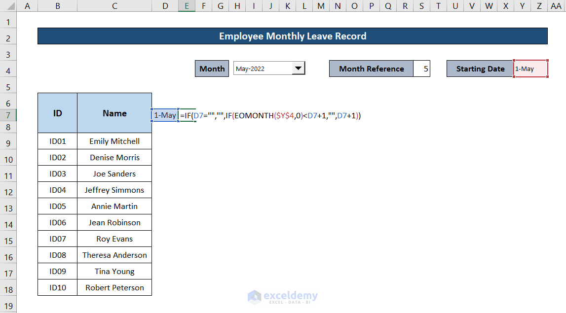
- Select cell D7 and insert the following formula in it.
=Y4
- Select cell E7 and copy the following formula in it:
=IF(D7="","",IF(EOMONTH($Y$4,0)<D7+1,"",D7+1))
Breakdown of the Formula
IF(D7=””,””,IF(EOMONTH($Y$4,0)<D7+1,””,D7+1))
(EOMONTH($Y$4,0) returns the last date of the month value in cell Y4.
IF(EOMONTH($Y$4,0)<D7+1,””,D7+1) checks if the previously mentioned function is equal or less of that of cell D7(the left of the cell itself). If the condition is true, this function returns a string. Else, it returns the following number.
Finally, IF(D7=””,””,IF(EOMONTH($S$4,0)<D7+1,””,D7+1)) checks cell D7 contains empty string or not. If it does, it returns an empty string. Otherwise it moves on to the function previously discussed. This whole function ensures that our number of days ends at the exact number of month we have selected in the combo box.
- Select the cell again and drag the fill handle to cell AH7.
- Select the range D7:AH7 and press Ctrl + 1 to format it.
- Select the Number tab in the Format Cells box, and in the Type field of the Custom section, type in dd.

- Click on OK. The spreadsheet will look like this at this point.

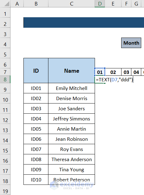
- Select cell D8 and insert the following formula.
=TEXT(D7,"ddd")
- Click and drag the fill handle icon to cell AH8 to make it look like this.
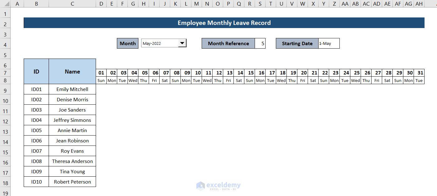
- Hide the month reference and starting date.
- Select the range D8:AH8 and press Ctrl + 1 to format.
- In the Format Cells box, go to the Alignment tab and select 90 degrees as orientation.

- Make the fonts bold.
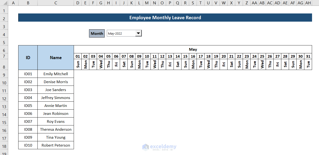
- Select the range D6:AH6 and select Merge & Center from the Alignment group in the Home tab.

- Insert the following in the merged cell and format it as an mmmm in the custom format box:
=K3
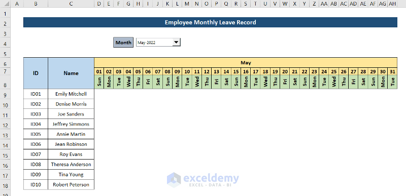
- Click on OK and the spreadsheet will now look like this.
- Fill it with color to make it more appealing.
- Select cell D9 and insert the following formula:
=IFERROR(VLOOKUP($B9&D$7,'Leave Table'!$B:$F,5,0),"")
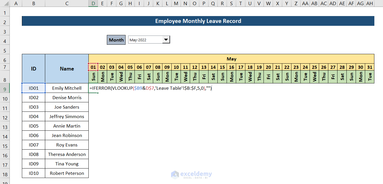
Breakdown of the Formula
IFERROR(VLOOKUP($B9&D$7,’Leave Table’!$B:$F,5,0),””)
VLOOKUP($B9&D$7,’Leave Table’!$B:$F,5,0)looks for value in range B9:D7 in columns B through F in the sheet called “Leave Table”. Argument “5” indicates the function will return a value from the fifth column. And the final argument “0” indicates it has to be an exact match.
The previous function is supposed to look for an exact match and return the value of the fifth column in the row it found the match. But there are cases where no match occurs. In case of that, we add the IFERROR portion of the formula. So that our charts’ cells won’t fill up with error warnings. The IFERROR(VLOOKUP($B9&D$7,’Leave Table’!$B:$F,5,0),””) formula returns an empty string if the value doesn’t match the VLOOKUP function.
- Press Enter and you will have the cell automatically filled up from the data of the previous spreadsheet.

- Fill the formula for the whole chart by clicking and dragging the fill handle icon vertically and horizontally.
- Fill in the cells after the chart as shown in the figure below.

- Select cell AI9 and input the following formula:
=COUNTIF($D9:$AH9,AI$8)
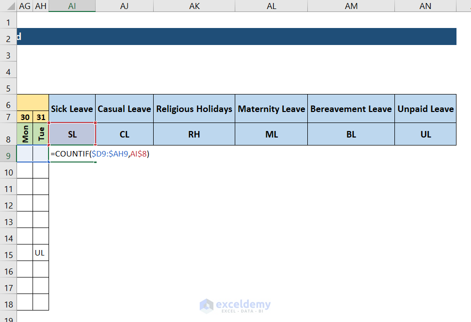
- Press Enter.
- Replicate the formula till the cell AN18 by first clicking and dragging the fill handle icon down and then to the right and you will have the chart to look something like this.
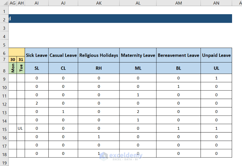
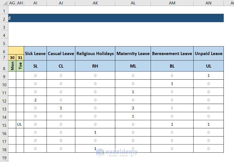
- Grey out the values with 0 to make the number of leaves stand out.
- Make a column for total leaves.

- Select cell AO9 and Insert the following formula in it.
=SUM(AI9:AN9)
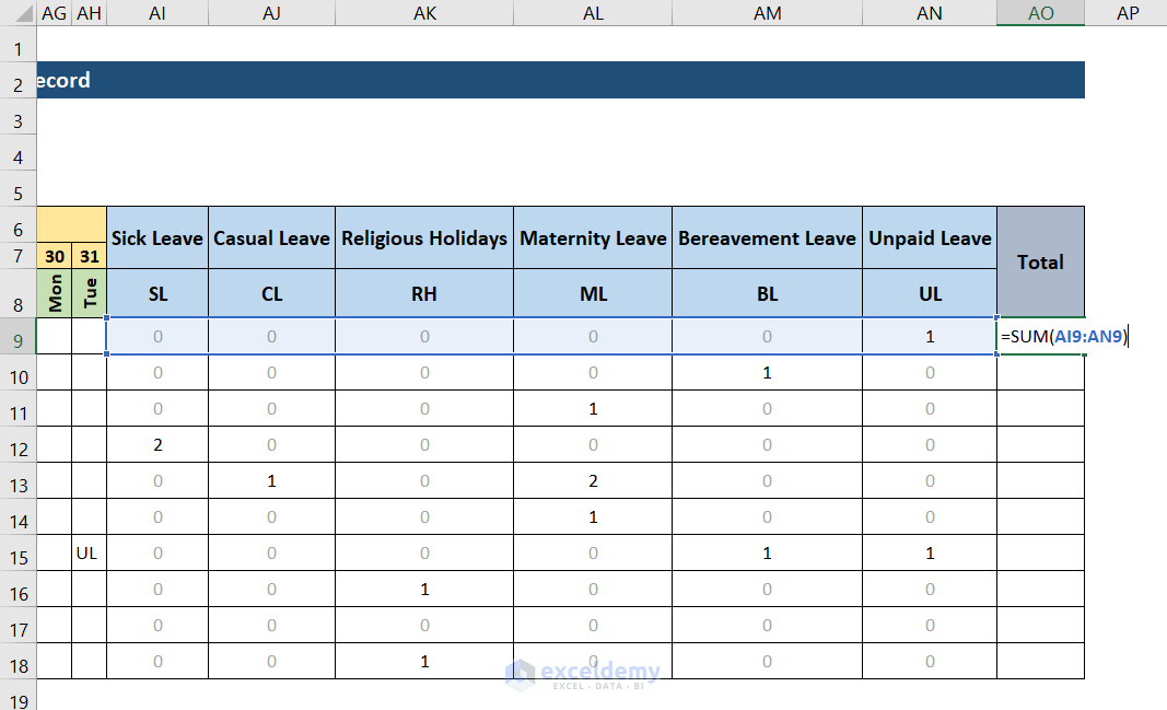
- Press Enter and you will get the total leaves taken by the first employee.

- Drag the fill handle icon down to replicate the formula for the other cells in the column.
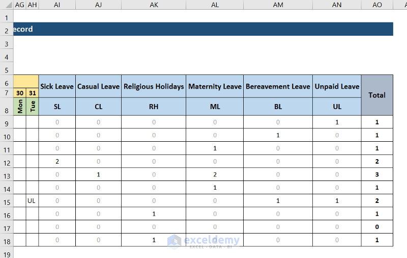
- Our final employee leaves record format will look something like this.
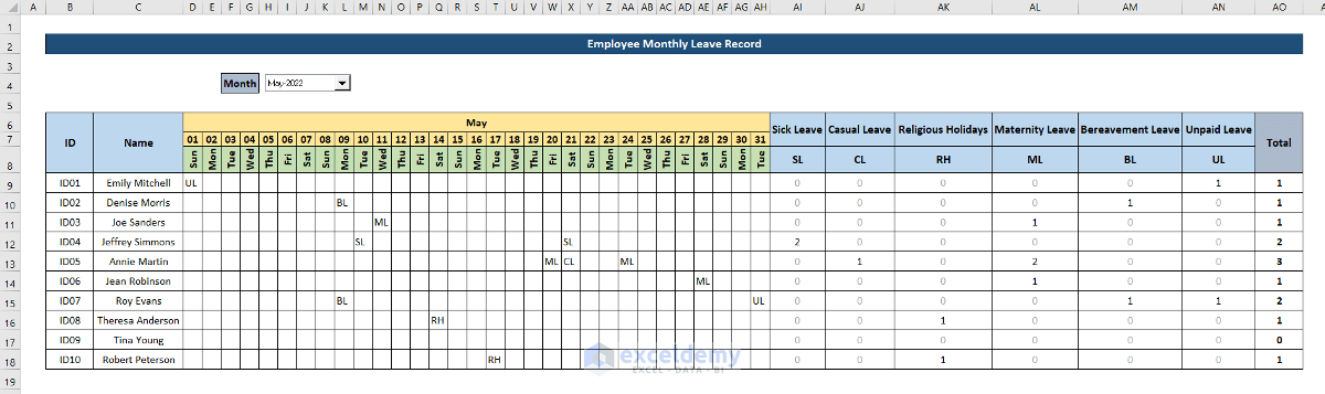
- Name the spreadsheet “Leave Calendar” as it represents a monthly calendar.
- You can also change the month from the combo box we have added and data entered in the “Leave Table” will automatically update the data to the appropriate month.
Read More: How to Track Employee Vacation Time in Excel
Step 4 – Verify the Employee Leave Record with Data
- Enter data in the spreadsheet we have created in step 2 called “Leave Table”.

- We can see from the list above that he had already taken two sick leaves prior to this. They have previously taken two leaves.
- Go back to the employee monthly leave record format we have created in the same Excel workbook in step 3.
- The value is updated.

Read More: How to Create Maternity Leave Calculator in Excel
Step 5 – Generate a Final Report
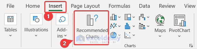
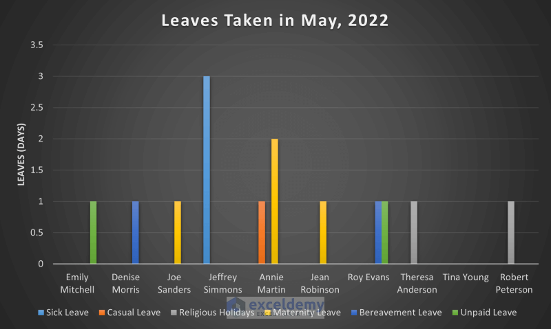
- Select three ranges, B6:C18 and AI6:AN18, in the “Leave Calendar” by holding Ctrl on your keyboard and clicking and dragging with the mouse.
- Go to the Insert tab on your ribbon and select Recommended Charts from Charts
- The Insert Chart box will pop up. Select the All Charts tab in it.
- On the right side of the box, select Column.
- Select the chart you prefer from the right side of the box.

- Click on OK, and you will get a graph on top of the spreadsheet.

- Make some modifications to make it more pleasing and we will have our final product.
Download Free Template
You can download the workbook used for the demonstration of the step-by-step guide from the link below. You can also use this as a template for your customized dataset.
<< Go Back to Excel Employee Leave Tracker | Excel HR Templates | Excel Templates
Get FREE Advanced Excel Exercises with Solutions!
