How to Track Employee Vacation Time in Excel: 7 Methods

Method 01 – Inserting the Name of the Month to Track Employee Vacation Time in Excel

• Select cell F2. Write down the formula below and press ENTER.

Formula Breakdown:

This formula returns the sheet name in the selected cell.

• CELL(“filename”,A1): The CELL function gets the complete name of the worksheet
• FIND(“]”,CELL(“filename”,A1)) +1: The FIND function will give you the position of ] we’ve added +1 because we require the position of the first character in the name of the sheet.
• 255: Excel’s maximum word count for the sheet name.
• MID: The MID function uses the text’s position from start to end to extract a specific substring.

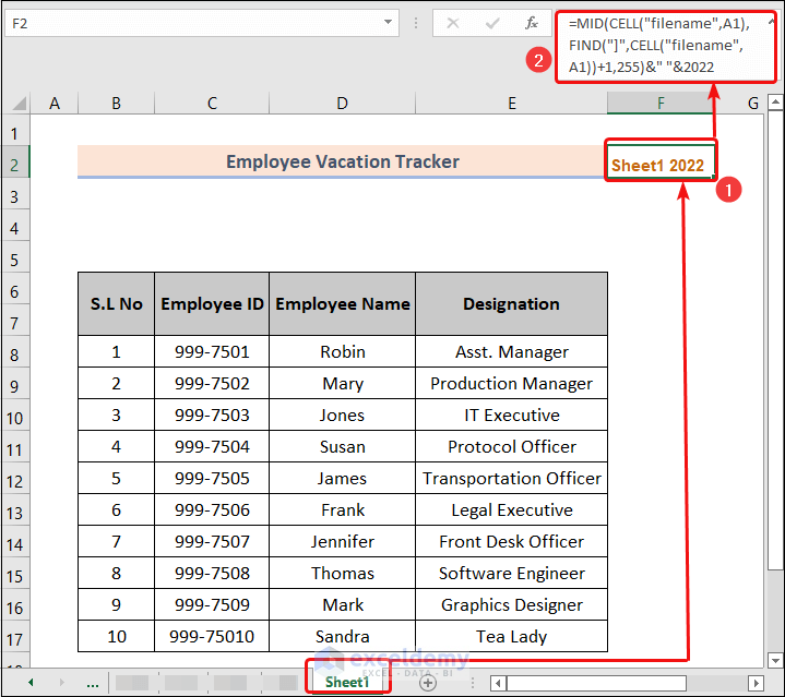
We can see the name of our Sheet on this cell with 2022.

Note: While typing this formula, make sure to enter any cell references on this sheet. Otherwise, the formula won’t work properly. For example, here we’ve entered the reference of cell A1.

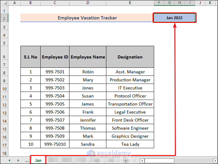
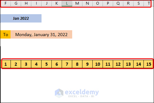
• Change the name of the sheet to Jan. Make the employee vacation sheet for the month of Jan’22. See that the month’s name is automatically input into cell F2 after changing the Sheet Name.

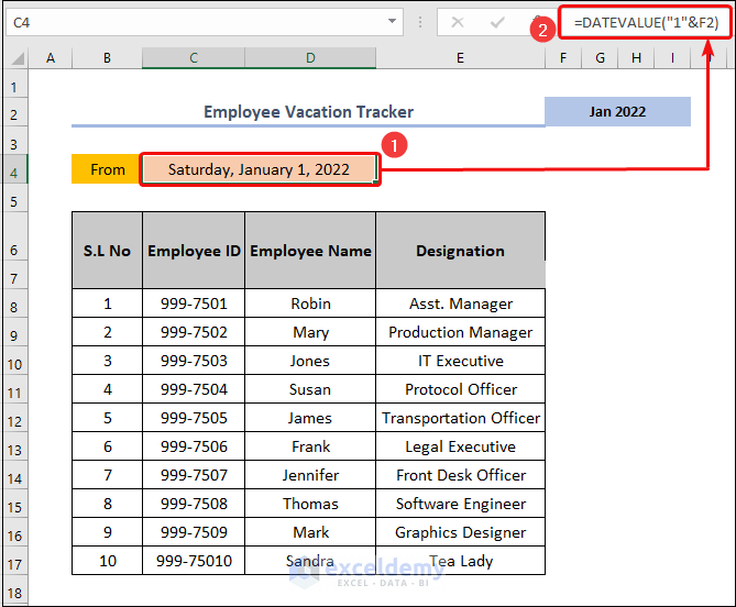
• We have to set the starting date for this month. Select cell C4 and input the formula below.

F2 represents the month of Jan 2022.

A date that is stored as text can be changed into a serial number that Excel can identify as a date using  the DATEVALUE function. Use the Custom Format option to show the date as in the image below.

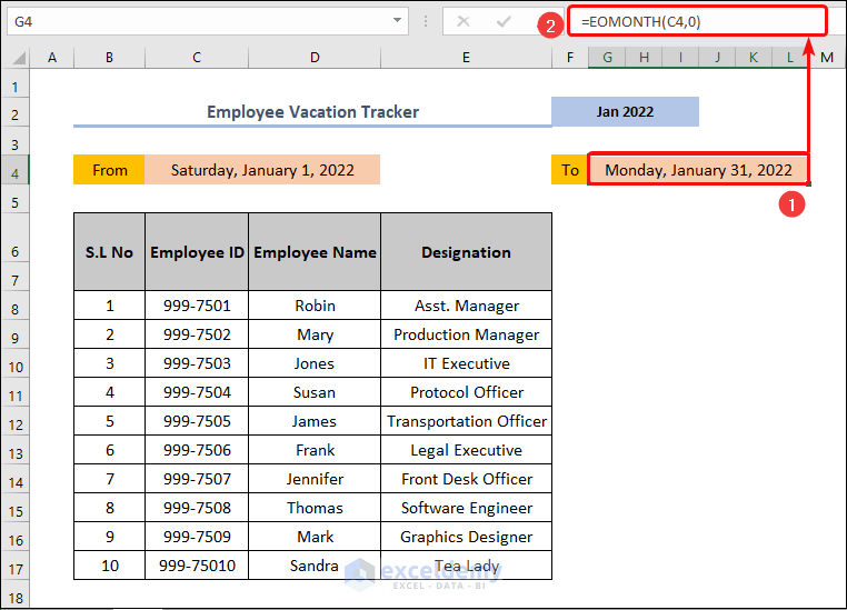
• Select cell G4 to show the ending date of that month. Write down the formula in the cell and press ENTER.

C4 represents the starting date of the month.

The EOMONTH function is used to determine the end of the month.

Method 02 – Creating Individual Date and Day

• Select cell F7. Type the formula below and press ENTER.

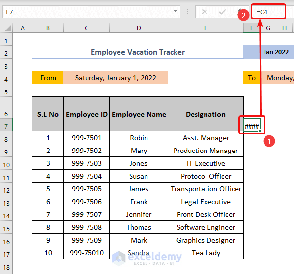
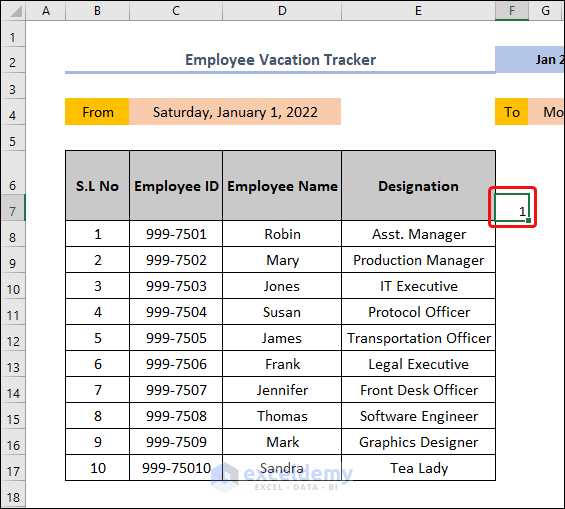
• Press CTRL + 1 to open the Format Cells wizard. Select Custom and type d in the Type box. Click OK.

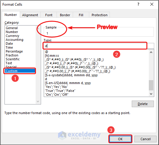
• The date looks like the image below.

• To input the second date, select cell G7. Write the formula below and press ENTER.

F7 and G4 represent the first date of the month and the last date of the month.

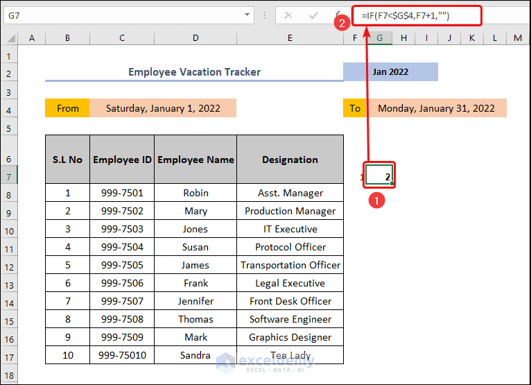
Formula Breakdown:

We’ve applied a logical test using the IF function here. If the date in cell F7 is less than the month’s end date, then the formula returns the next date from the date in cell F7. Otherwise, it will show nothing.

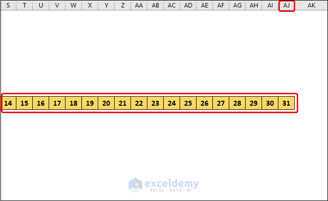
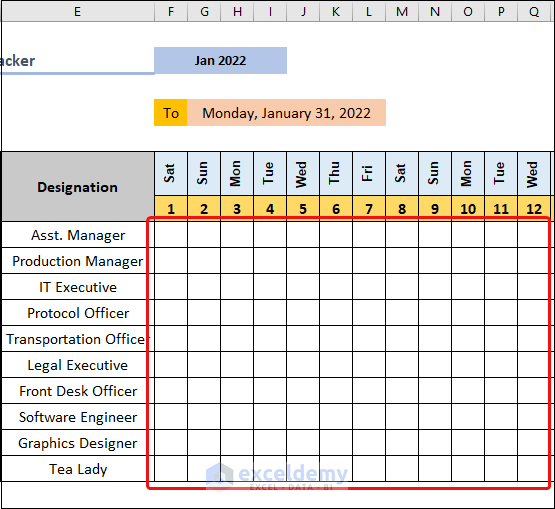
• Use the Fill Handle tool and drag it to cell AJ7 to exhibit the remaining days of the month.

• Select the columns in the F: AJ range. Go to the Home tab. Select Cells > Format > Column Width.

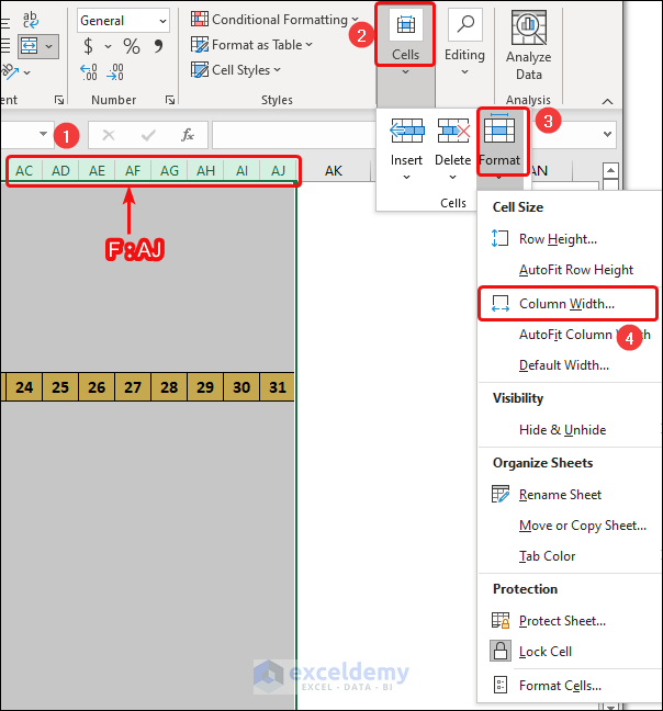
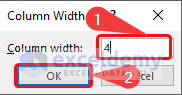
• Type 4 in the Column Width box and click on OK.

• Have our column at the perfect width because we will just put V into these cells.

• Select cell F6 and type the formula below. Press ENTER.

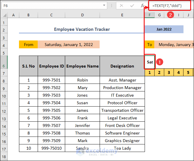
• Indicate the other days till the date of 31 using the Fill Handle Tool. From the Home tab, click on the small arrow in the Alignment group > write down 90 in the Degrees box and click OK.

• The name of the day rotates vertically with this action.

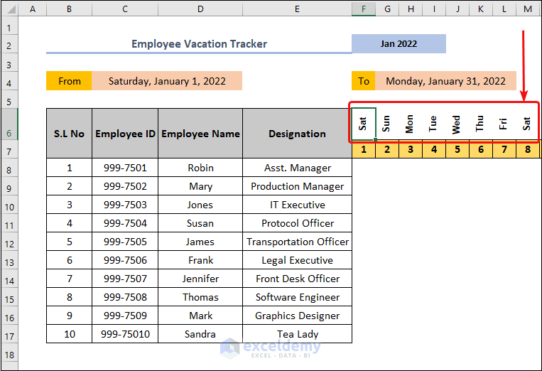
• Fill the cells with your preferred colors and apply All Borders to the cells.

Method 03 – Formatting Weekly Holidays

• Select cell F8. Then, go to the Home tab and select Conditional Formatting > New Rule.

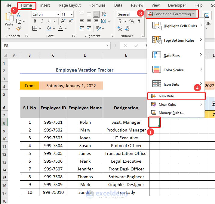
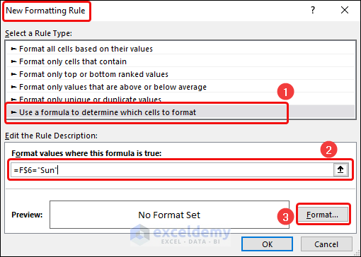
• The New Formatting Rule dialog box will open. Select the options as in the image below. Write the formula in the formula box and click on Format.

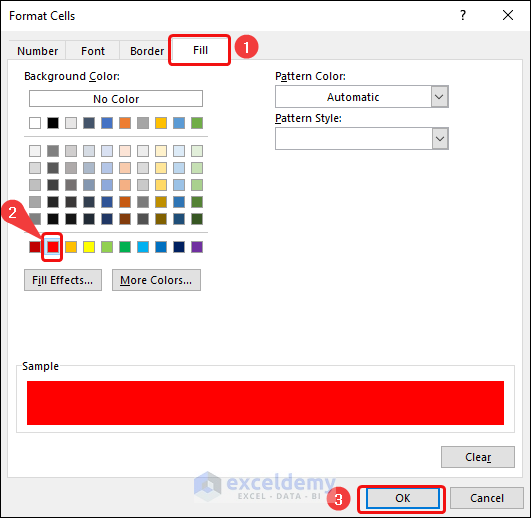
• The  Format Cells dialog box opens. After that, select the Fill tab > Choose your preferred color and click OK.

• It returns to the New Formatting Rule dialog box. Click OK.

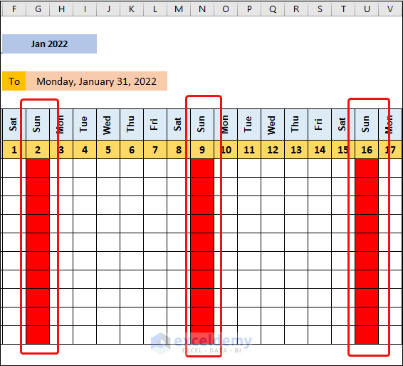
• Use the Fill Handle tool to expand this formatting in cells in the F8:AJ17 range. The cells under the columns of the Sun are highlighted in red.

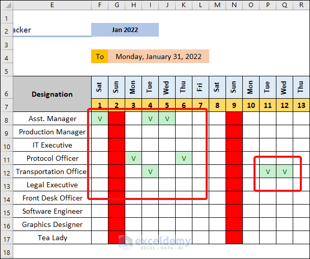
Method 04 – Inserting Vacation in Cells as V

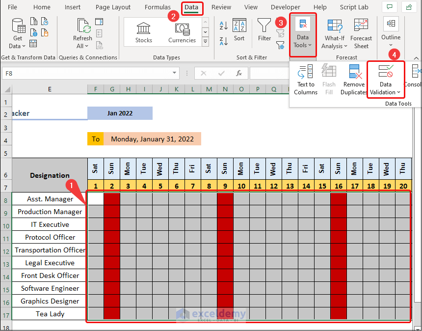
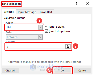
• Select cells in the F8:AJ17 range. Go to the Data tab and select Data Tools > Data Validation.

• The Data Validation dialog box opens. Go to Settings. Select List from the drop-down list in the Allow box. Write down V in the Source box. Now, click OK.

V means “vacation”.

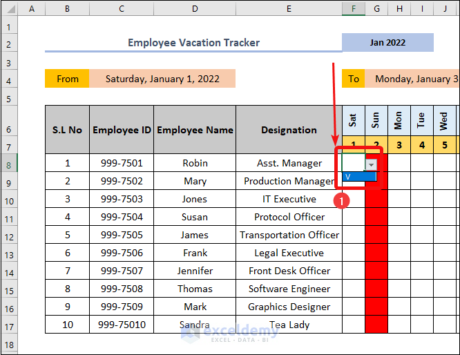
• Click on cell G8. You can see a drop-down list containing just V. That means we could just input this text only.

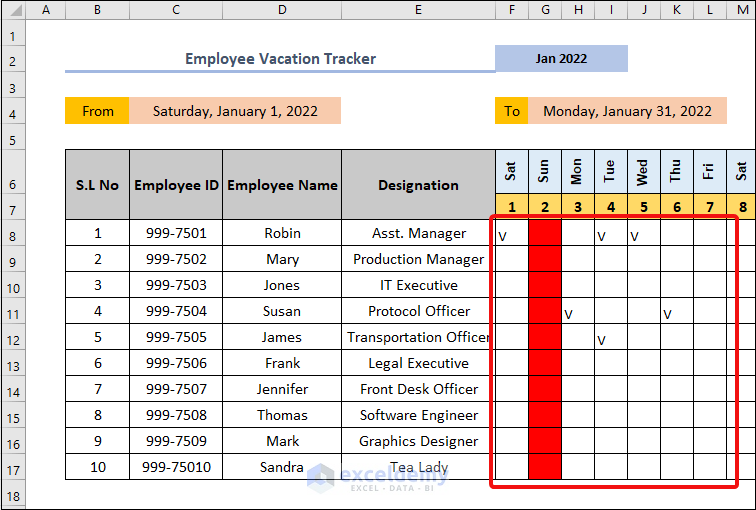
• Place the vacation days of all individuals in their respective cells. A portion of vacation marking is like below.

• Select the cells in the F8:AJ17 range. Go to the Home tab. Select Conditional Formatting > Highlight Cells Rules > Text that Contains.

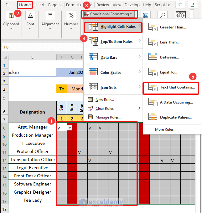
• In the Text That Contains dialog box, write down V in the Format cells that contain the text box. Choose the formatting as in the image below. Lastly, click OK.

• Cells containing V reflect the defined highlighting.

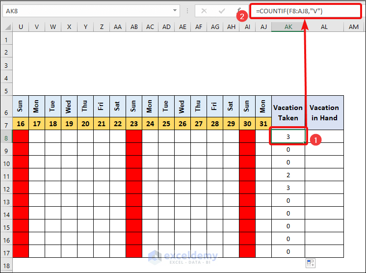
Method 05 – Counting Vacation Days and Vacations in Hand

• Select cell AK8 and type in the formula below. Press the ENTER key.

F8:AJ8 represents the cell range to input V.

We used the COUNTIF function to count V in the above range.

• Select cell AL8. Type the formula below and press ENTER.

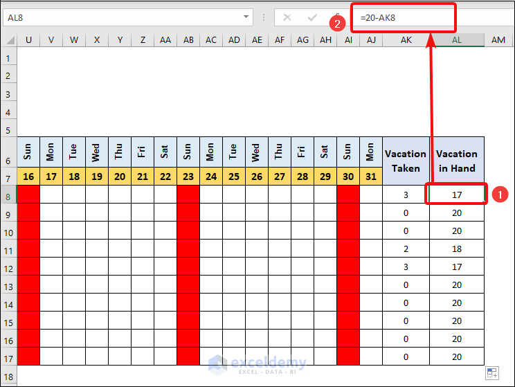
• Format the cells with effective colors to make the data more visible.

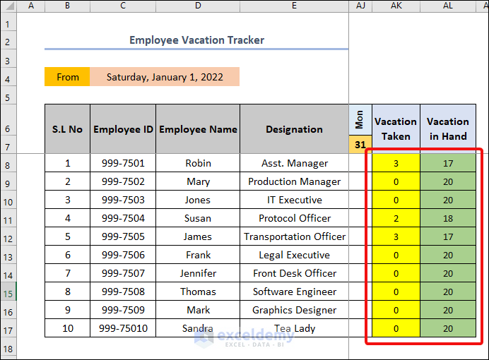
• Use the Freeze Panes tool to freeze the columns in the A:E range and freeze the rows in the 1:7 range. Select cell F8 first and go to the View tab. Select Window group > Freeze Panes drop-down menu > Freeze Panes tool.

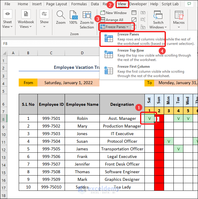
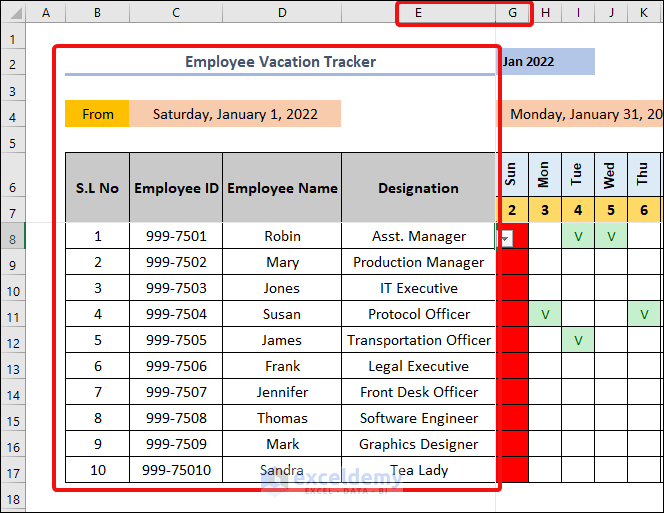
• The cells on the left and above F8 become frozen. It is very helpful as our sheet is expanded horizontally.

Method 06 – Following Steps 3-5 for Other Months

• Right-click on the Sheet Name of the Jan worksheet. Select Move or Copy.

• Select the options as shown in the image below and click OK.

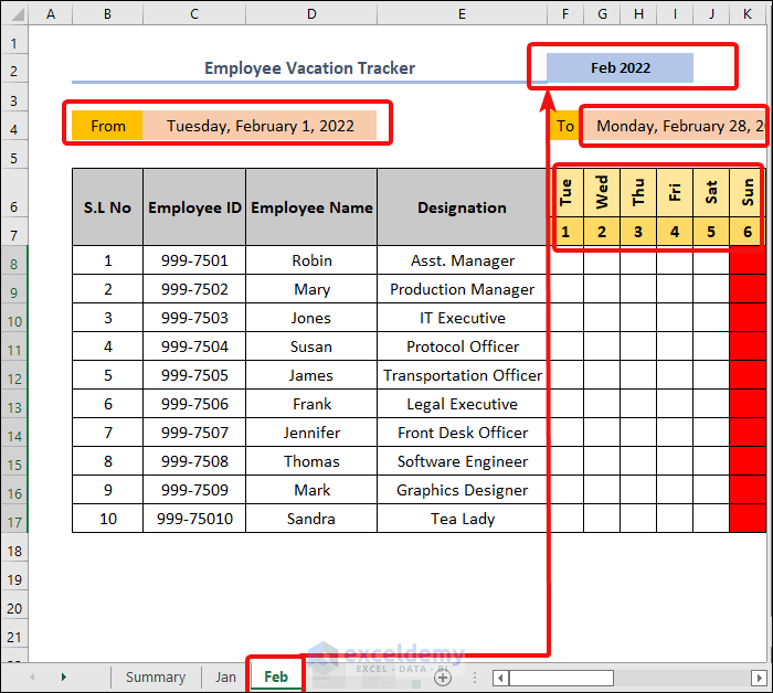
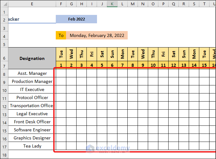
• Write down Feb in our 2nd Sheet Name. You can see that the worksheet is totally changed according to the February month. The weekly days were set up as consecutive dates. You will notice the start and end date of the month changed automatically.

• The Conditional Formatting again highlights the holidays. We’ve got to do it manually for each sheet.

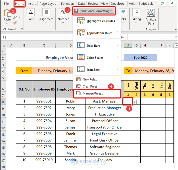
• Select cell F8. Then, go to the Home tab and select Conditional Formatting > Manage Rules.

• The Conditional Formatting Rules Manager opens. Choose This Worksheet from the Show formatting rules for list, and select the range to apply the formatting and click OK.

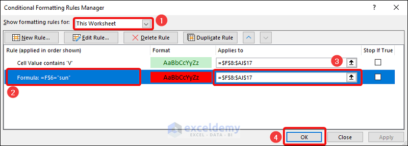
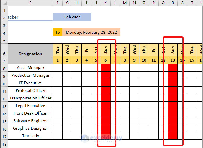
• We highlighted the weekly holidays again.

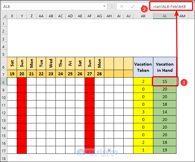
• There is a slight change in the formula for counting the Vacations in Hand in this worksheet. Select cell AL8 and write down the formula below. Press the ENTER key.

We are subtracting the Vacation Taken in February month from the Vacation in Hand of month January.

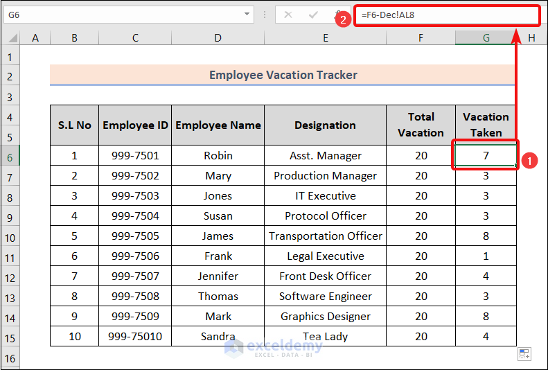
Method 07 – Creating a Summary to Track Employee Vacation Time in Excel

• We calculated the Vacation Taken in the year. Select cell G6 and write down the formula below. Press the ENTER key.

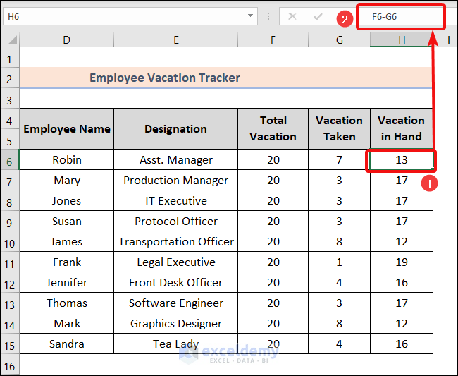
• We showed the Vacations in Hand at the present time. Select cell H6 and type the formula below. Press ENTER.

Benefits of Employee Vacation Time Tracker

As this tracker template is completely automatic, we don’t need to make a format for the month every time. Copy our created worksheet first and change the name of the worksheet to convert it into another month’s tracker.

Use this template for other years. We just have to edit the formula in cell F2.

In the above formula, just write 2023 in place of 2022. Magically, this template will be compatible until 2023.

This template is completely ready to use. Assign different Vacation days for individual employees. Edit the cells in the F6:F15 range in the Summary worksheet.

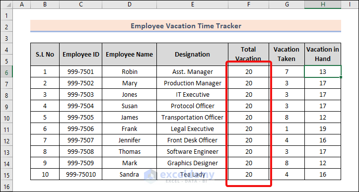
Besides these, you can add more employees according to your needs. Just use the Fill Handle tool to get results in those new cells.

So, what’s holding you back? Download the template now. Use it and turn the race in your favor.

Download Practice Workbook

You may download the following Excel workbook for better understanding and practice yourself.

Related Articles

• How to Create Employee Leave Record Format in Excel
• How to Create Maternity Leave Calculator in Excel

<< Go Back to Excel Employee Leave Tracker | Excel HR Templates | Excel Templates