How to Freeze Selected Panes in Excel (4 Suitable Examples)

Here’s an overview of where you can find the Freeze Panes options.

Download the Practice Workbook

How to Freeze Selected Panes in Excel: 4 Examples

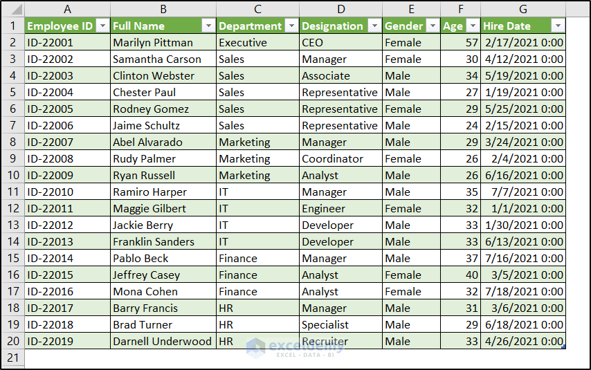
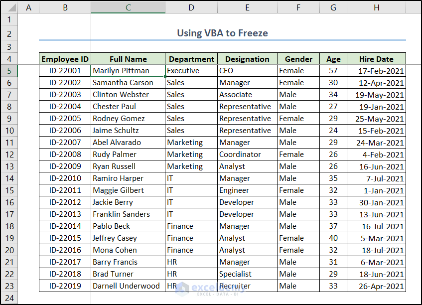
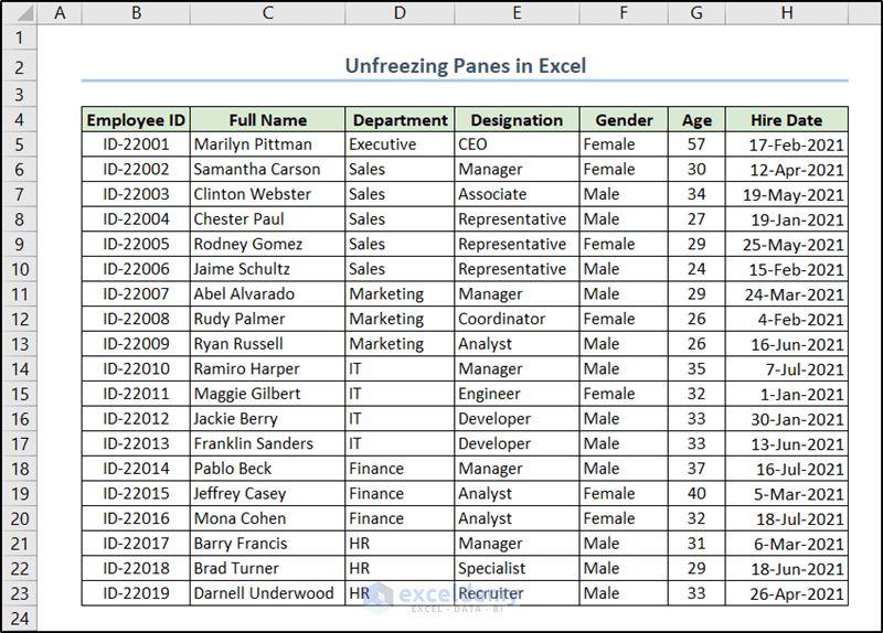
The sample dataset contains a list of employees with their IDs and other information. We will freeze different portions so certain information stays on the screen while scrolling.

Example 1 – Freeze Either Selected Rows or Columns Individually in Excel

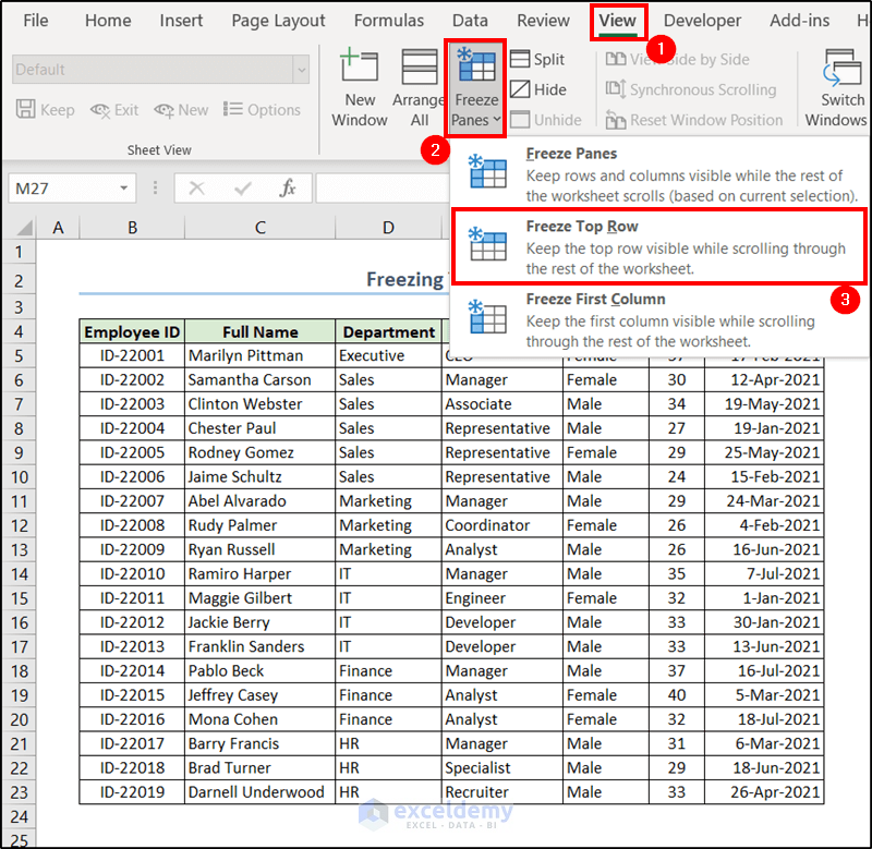
Case 1 – Freeze the Top Row

Go to the View tab and select Freeze Panes from the Window group.
Select Freeze Top Row.

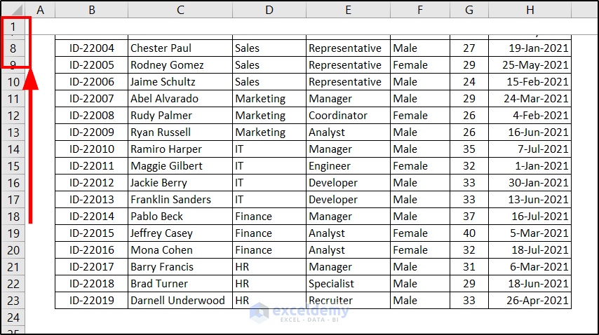
You will notice a grey line appearing below the first row.

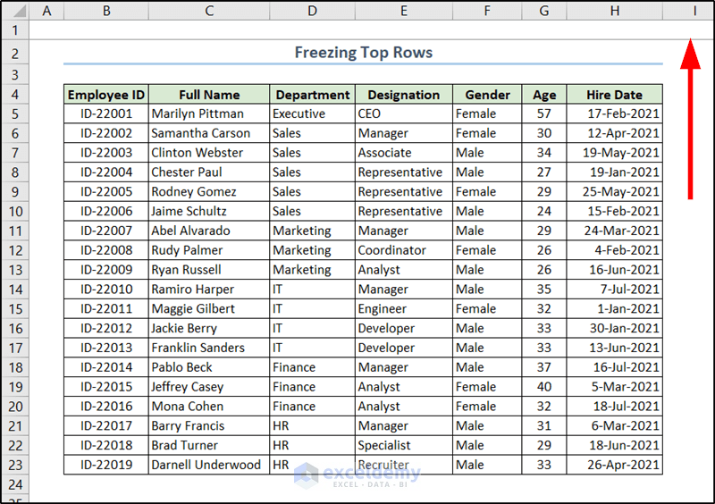
When you scroll down, the first row is always on the screen.

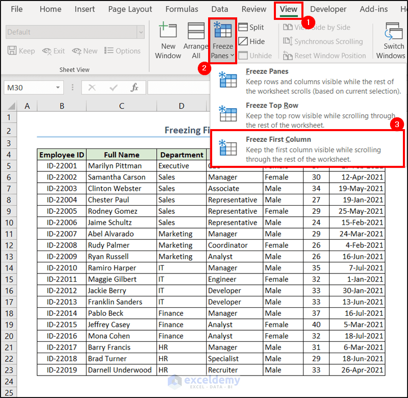
Case 2 – Freeze the First Column

Go to the View tab and, from the Window group, select Freeze Panes.
Select Freeze First Column from the drop-down menu.

You’ll get a vertical line between columns A and B.

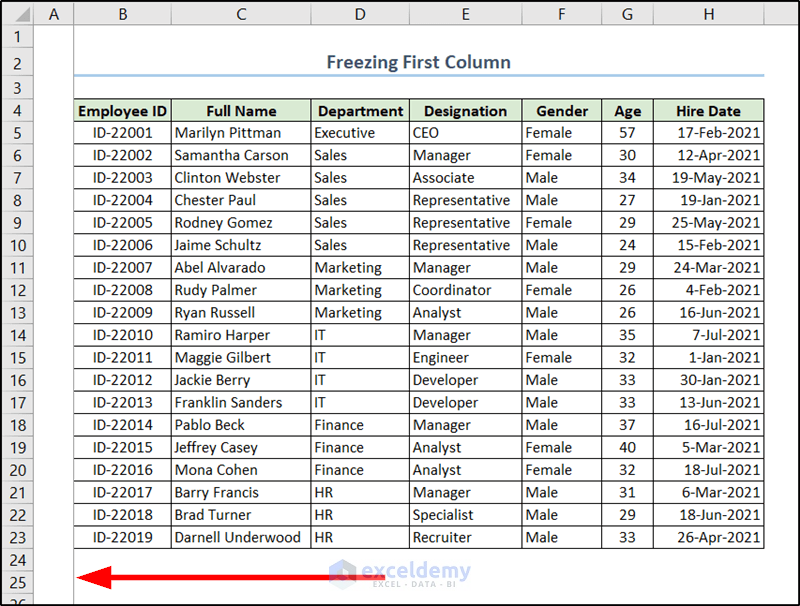
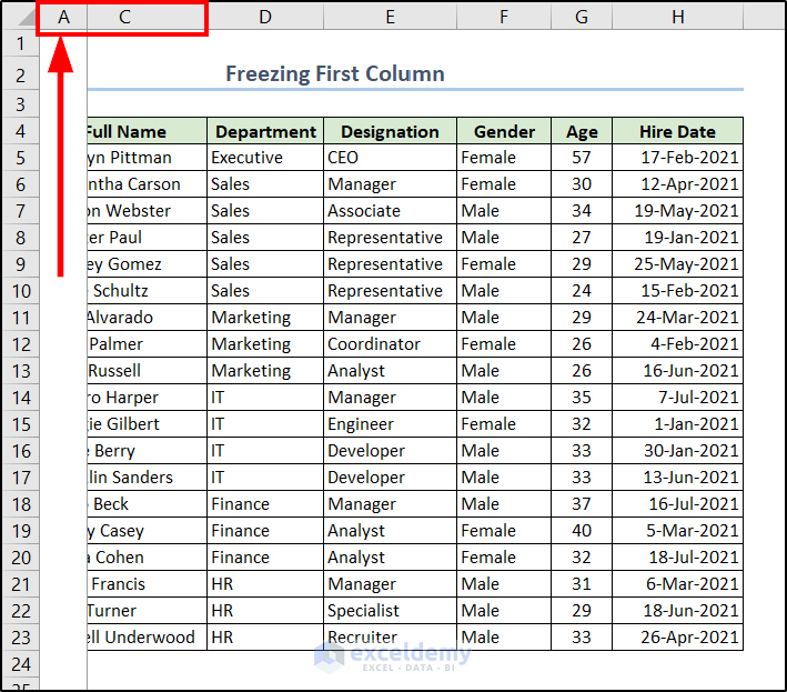
If you scroll to the right, the first column will always be there.

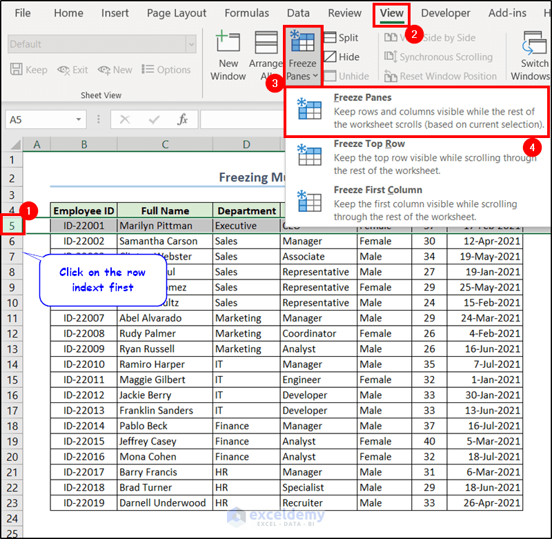
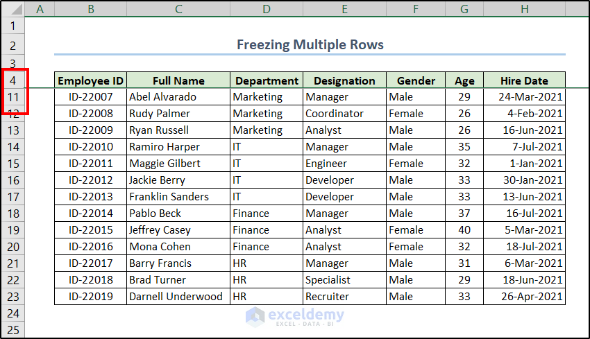
Case 3 – Freeze Multiple Rows

We want to freeze the headers and the dataset title, which are the first four rows in the sample spreadsheet.

Select the fifth row (the row after the freezing should end) by clicking on the row index on the left of the spreadsheet.
Go to the View tab and select Freeze Panes from the Window group.
From the drop-down menu, select Freeze Panes.

The grey line appears between rows 4 and 5. Scroll down the sheet and you will see the first four rows are frozen.

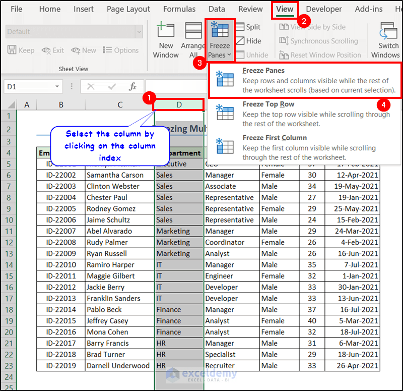
Case 4 – Freeze Multiple Columns

We want to freeze the “Employee ID” and “Full Name” columns (so columns B and C).

Select column D (the first one that should not be frozen).
Go to the View tab and select Freeze Panes from the Window group.
From the drop-down menu, select Freeze Panes.

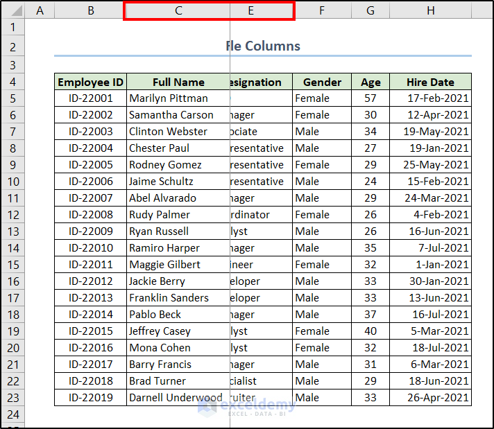
The grey line will appear vertically after C. If you scroll to the right, the first three columns won’t move

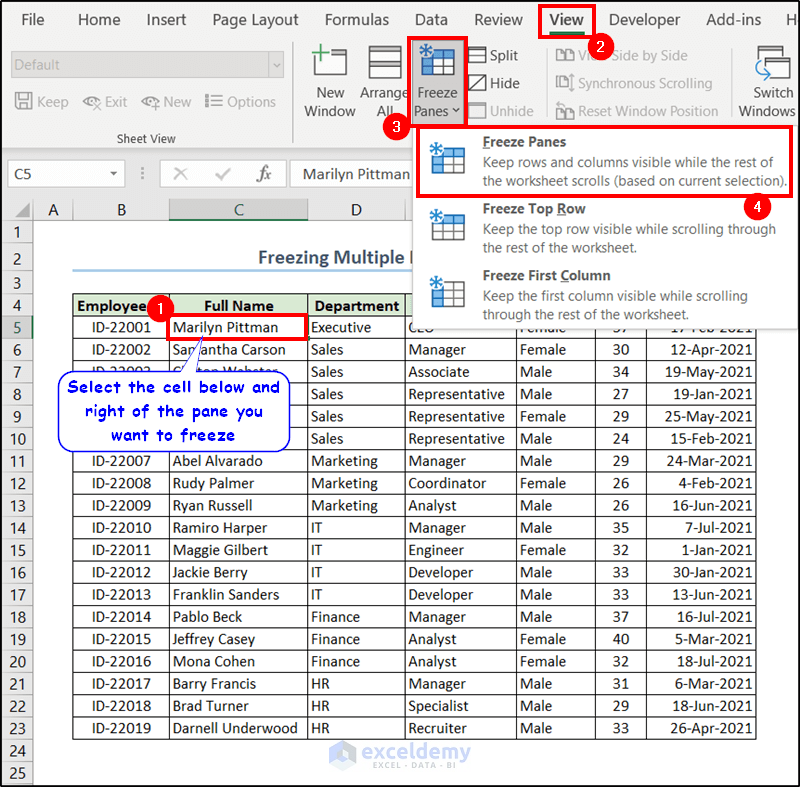
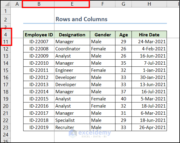
Example 2 – Freeze the Selected Columns and Rows at the Same Time

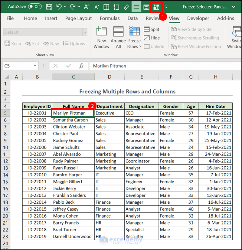
We’ll freeze the top four rows and the top two columns in the sheet.

Select the cell below and on the right of the row and column you want to freeze. In this case, that’s cell C5.
Then select Freeze Panes from the Window group of the View tab.
From the drop-down menu, select Freeze Panes.

You’ll get two grey lines, one after row 4 and the other after column B. Scrolling will keep the frozen rows and columns in view.

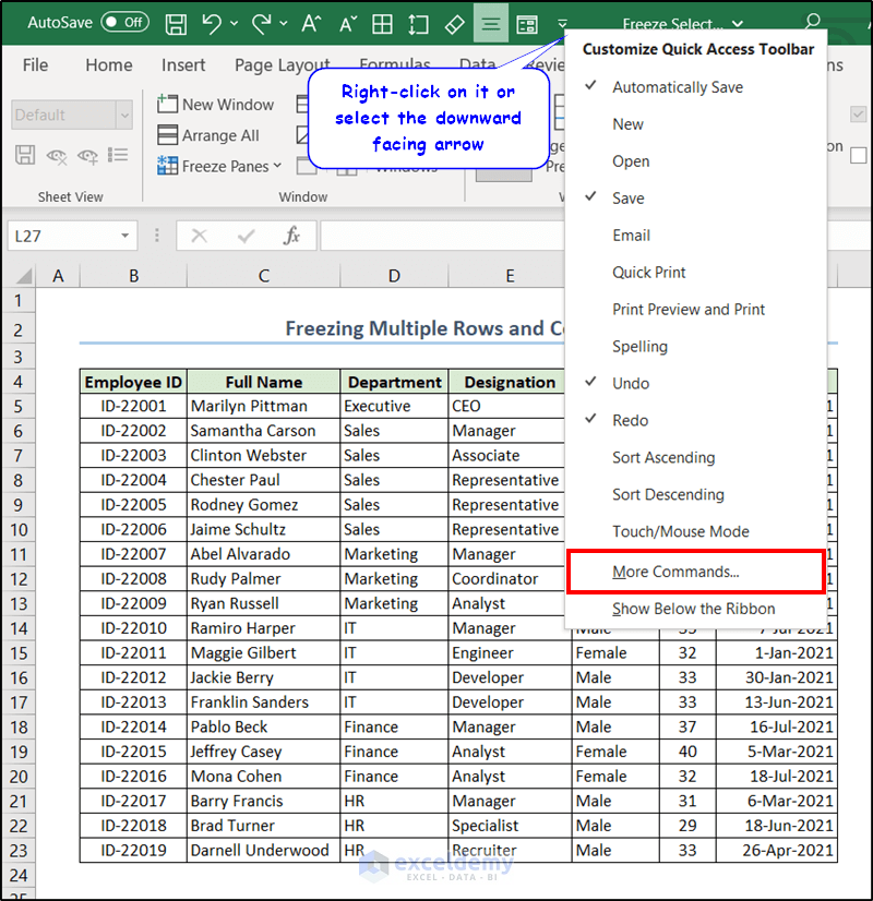
Part 2 – Add the Freeze Panes Button to the Quick Access Toolbar

Right-click on the Quick Access Toolbar on top of the Excel window and select More Commands from the context menu.

Select the Quick Access Toolbar tab in the Excel Options box.
Under the Choose commands from option, select Commands Not in the Ribbon.
On the list on the left, select the Freeze Panes option and select Add.

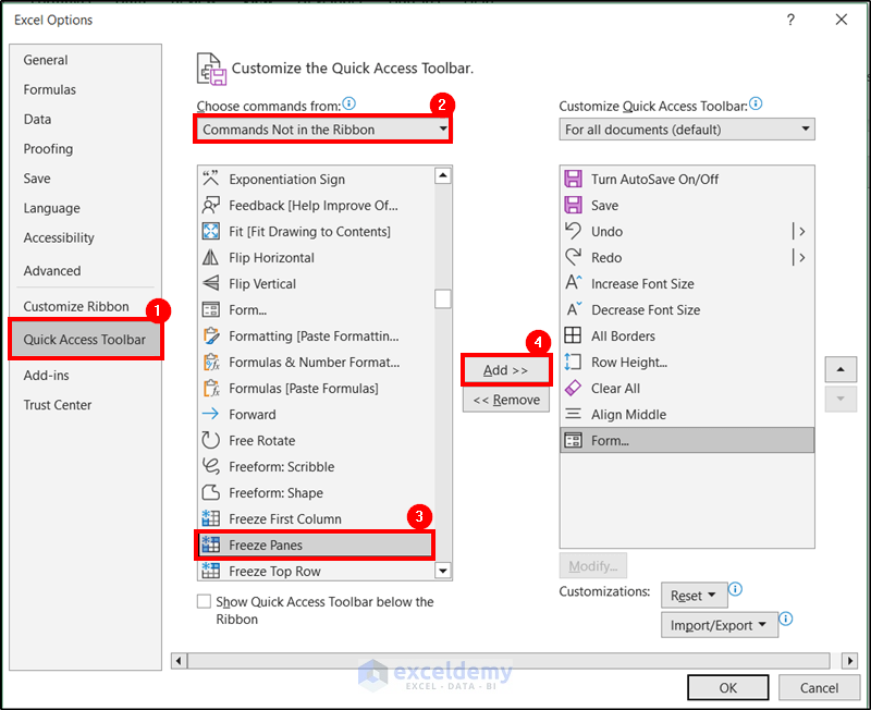
Click on OK and the Freeze Panes button will be available in the Quick Access Toolbar.
Select the cell below and to the right of the pane you want to freeze and click on the button to freeze selected panes in the Excel spreadsheet.

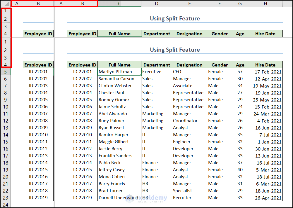
Example 3 – Freeze Selected Panes Using the Split Feature and Get Frozen Panes Twice

We are going to freeze (or split) the column headers and the “Employee ID” column.

Select the cell below and right of the pane you want to freeze. In this case, it is cell C5.
Go to the View tab.
Select Split from the Window group.

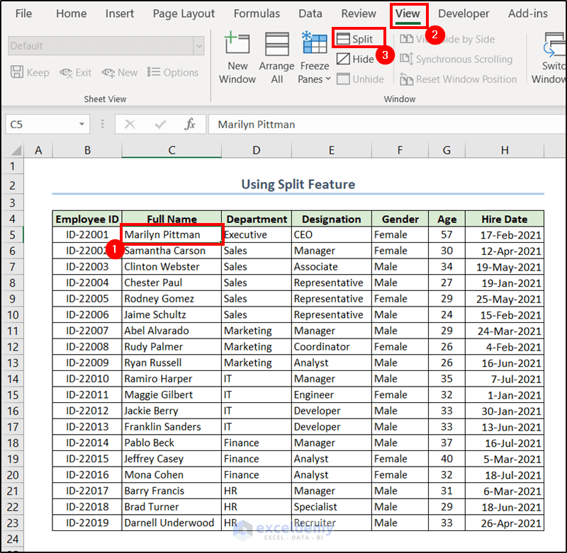
You will see the grey lines appearing on the top and left of the cell we selected. If you scroll down or to the right, this will freeze selected panes in the Excel spreadsheet.

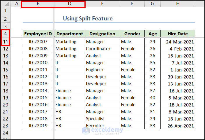
However, if you scroll up or to the left, you may see the panes appearing twice.

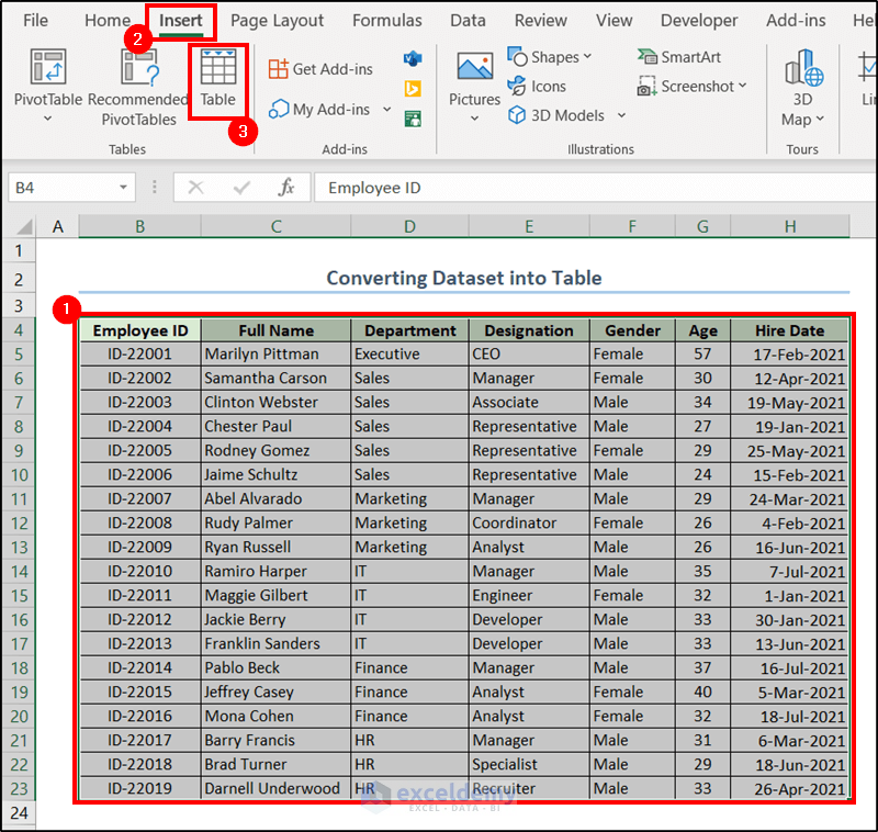
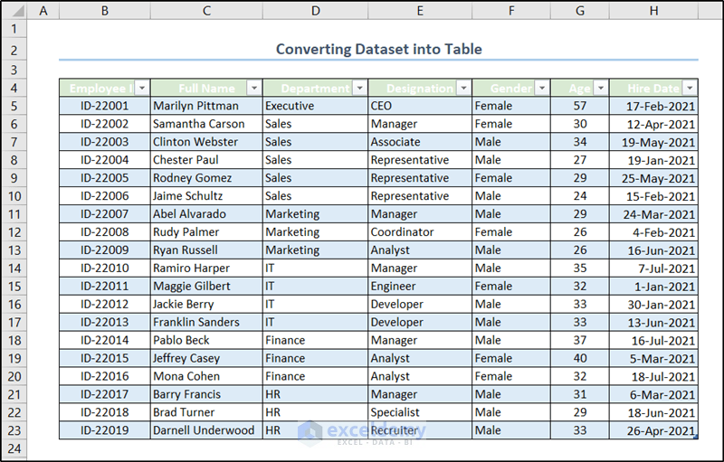
Example 4 – Freeze Column Headers by Converting the Dataset into an Excel Table

Select the dataset and go to the Insert tab on the ribbon.
Select Table from the Tables group.

A Create Table box will open. Make sure the correct range is in the field and check the My table has headers option, then click OK.

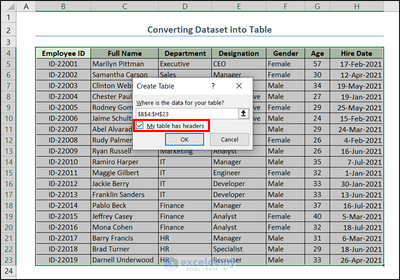
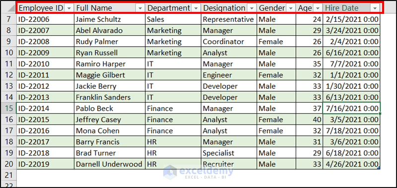
The dataset will now convert into an Excel table with filters on the headers.

If you scroll down while selecting a cell on the table, you will see the column headers on the column index.

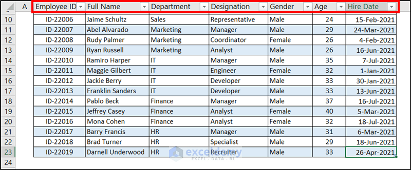
This will work as long as you have selected a cell from the table. If you select a cell outside the table and scroll down, you’ll see the original column indexes instead.

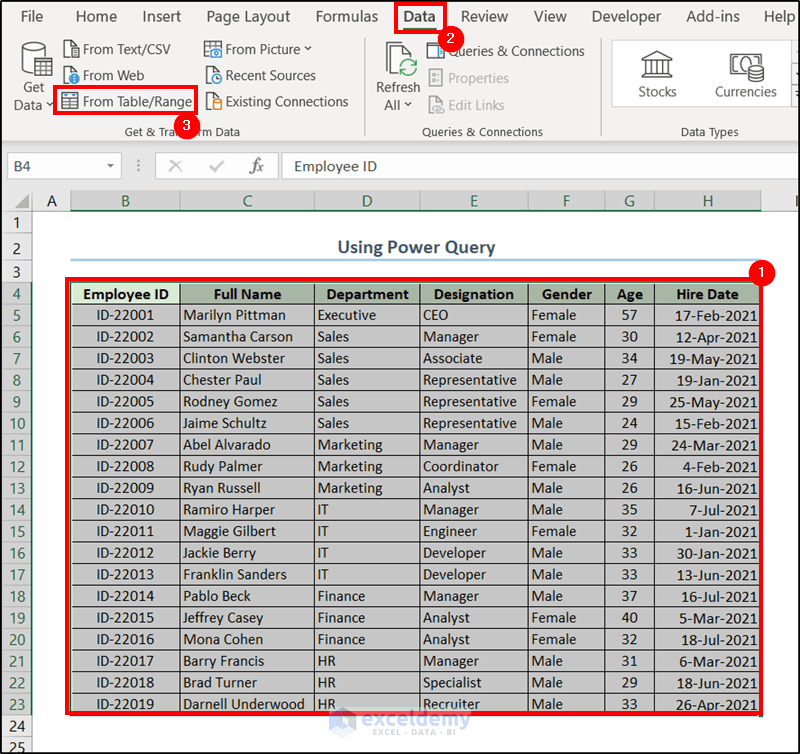
Part 2 – Converting to a Table via Power Query

Select all cells in the dataset.
Go to the Data tab on the ribbon and select From Table/Range from the Get & Transform Data group.

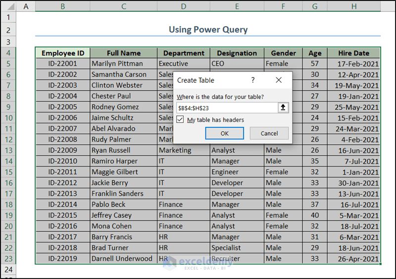
Insert the dataset range if needed and check the header option in the box and click on OK.

The Power Query window will open.
Click Close & Load.

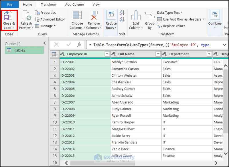
A table will appear on a new sheet with the filters on the headers just like how we find them on Excel tables.

You can scroll down and see the headers are frozen on the column index as long as a cell is selected in the table.

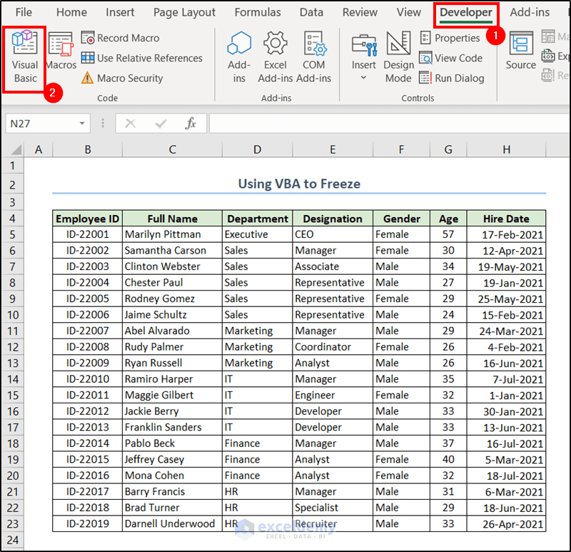
Alternative: Using VBA Code to Freeze Selected Panes Quickly

Visual Basic for Application (VBA) is a programming language available in Microsoft Office applications. We can use it for simple tasks such as selecting a cell or to automate repetitive complex tasks.

You need the Developer tab to show on the ribbon first. If you don’t have one, you can check out how to display the Developer tab on the ribbon.

Go to the Developer tab and select Visual Basic from the Code group of the ribbon.

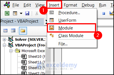
The VBA window will open up. Select the Insert tab and click Module from the drop-down.

In the module, insert the following code.

Sub freezepanes()

Range("C5").Select
ActiveWindow.freezepanes = True

End Sub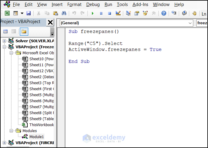

Press F5 to run the code. It will freeze the listed panes (assigned with cell C5) from the code in the current Excel spreadsheet.

Note: To freeze other panes, change the cell inside the range of the code to the one below and right of the pane.

How to Unfreeze Selected Panes in Excel

Select the sheet where you want to unfreeze and go to the View tab on the ribbon.
Select Freeze Panes.
Select Unfreeze Panes from the drop-down menu.

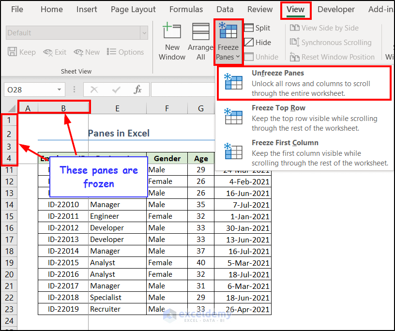
This will unfreeze all panes in the sheet.

Note: Pressing Ctrl + Z will not undo the Freeze Panes or Unfreeze Panes commands.

Freeze Panes Not Working in Excel

You are in cell editing mode: This is when you enter values in the cell. Any key you press on your keyboard at this point enters a value in the cell. Press Esc to exit this and the Freeze Panes command should work again.
Your spreadsheet is protected: Spreadsheet owners sometimes protect their sheets before sharing to avoid further editing of the sheet. In this case, you can’t edit or freeze cells. To unprotect them, go to the Review tab > select Unprotect Sheet.
Multiple Windows: Sometimes the Freeze Panes command behaves unnaturally because there are multiple windows of Excel running. In that case, close additional windows and try freezing the panes again.

Frequently Asked Questions

What happens if I delete or modify the frozen rows or columns?

If you have multiple rows or columns frozen, the number of frozen ones will decrease by one. But if you have one row or column in the pane, the 2nd row or column will shift to the frozen pane.

Can I freeze panes in a selected range, instead of the entire worksheet?

You can freeze panes from the start of the row (or column) to any of the preferred ones. However, you can not freeze some rows or columns in the middle and scroll both sides as in the current version of Excel.

Can I freeze panes in Excel without using the ribbon or menu options?

You can use the Quick Access Toolbar to add a freeze button. Or you can use VBA. Otherwise, you need to visit the ribbon.

Things to Remember

Pressing Ctrl + Home (which usually takes you to the first cell of the sheet) takes you to the first cell of the unfrozen row in a spreadsheet where the Freeze Panes option was used.
If you press Ctrl + End you will get to the end cell of the dataset for both sheets with frozen and unfrozen panes.
Always select the cell below and right of the pane you want to freeze. Consider it as the intersection of the first unfrozen column and row.
Converting a range into a table will only freeze the headers.
Ctrl + Z will not undo the freezing/unfreezing operation.
The freezable rows/columns always start from the first to the previous of what you select.

Get FREE Advanced Excel Exercises with Solutions!