How to Freeze Top Two Rows in Excel (4 ways)

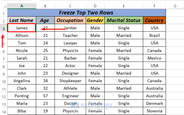
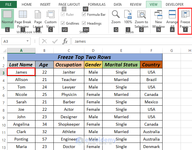
To put the concept of freezing the top two rows into practice, here’s a sample data set of people’s basic information: Last Names, Ages, Occupations, Marital Status, Gender, and Country.

Method 1: Freeze Top Two Rows Using View Tab

Excel has a few built-in features to freeze any number of rows or columns. For the example dataset, freezing the top two rows allows you to keep track of both column headers. So, the question is, how you will do this? Follow these steps to learn the process:

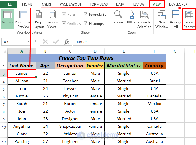
1. Click below the cell where you want to freeze the rows. For this dataset, click on cell A3.
2. Go to the View tab and click the Freeze Panes option.
3. Click the Freeze Panes option from the dropdown.
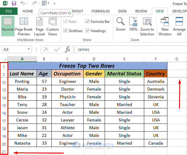
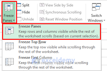4. After that, the dataset will look like the following image.

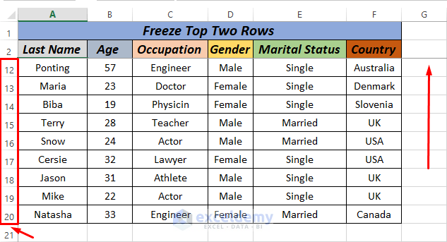
You can see the top two rows got frozen by scrolling down to the 20th row while the first two remain visible. For this method to work properly, make sure that you select the first cell in the third row. If you selected B3, for example, you’d also freeze the first column.

Read More: How to Freeze Top Row in Excel

Method 2: Freezing Top Two Rows Using Shortcut key

You can also use a shortcut key to freeze the top two rows in a sheet:

1. First, select the cell A3 since you’re freezing the rows above this cell.
2. Then, press ALT + W to enter the View tab. After that, Excel will show further keyboard prompts.
3. Press F to enter the Freeze Panes section.
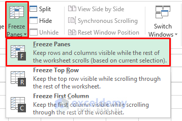4. Hit F again to select Freeze Panes from the options.

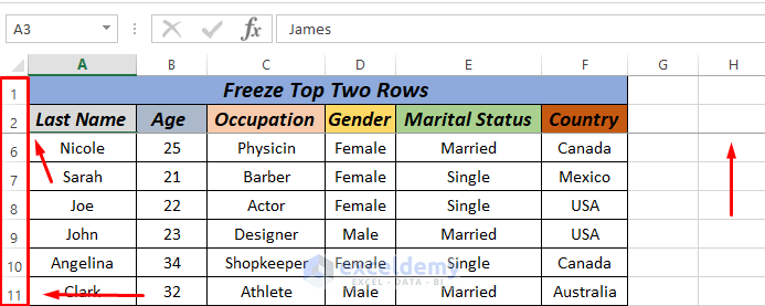
If you look closely, there is a horizontal line in row 2 indicating that the rows above that line are frozen.

So, the entire keyword shortcut is ALT W F F.

Read More: How to Freeze Top 3 Rows in Excel

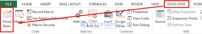
Method 3: Freeze Top Two Rows in Excel Using VBA

You can also use Excel VBA coding to freeze top two rows. Here is how:

• Press Alt + F11 on your keyboard or go to the tab Developer -> Visual Basic to open the Visual Basic Editor.
• In the pop-up code window, select Insert -> Module.
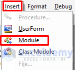• Copy the following code and paste it into the Module.

Sub FreezingTopTwoRows()
    Rows("3:3").Select 
ActiveWindow.FreezePanes = True 
End Sub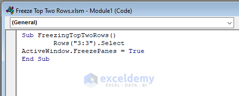

• Via this code, we are telling Excel to freeze rows above row 3:3.
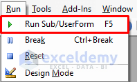
• The code is now ready to run. Press F5 on your keyboard, or go to the menu bar on the top and select Run -> Run Sub/User Form. You can also just click on the Small Play Icon in the sub-menu bar to run the macro.
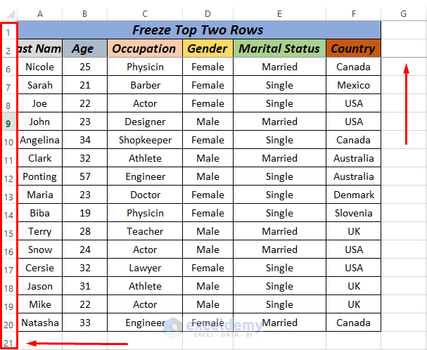
• Go back to the sheet and check if the two top rows are indeed frozen by scrolling down.

Read More: How to Freeze Columns in Excel

Method 4: Freeze Top Two Rows By Magic Freeze Button

This method allows you to add the Freeze Panel button in the quick access bar and freeze the top two rows in Excel quickly:

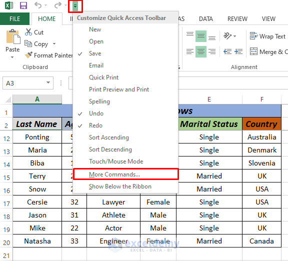
1. First, go to the top of the worksheet and click on the down arrow.
2. Go to More Commands…, as the following image shows.
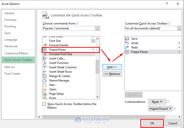
3. A new dialogue box will pop up.
4. Select the Freeze Panes option and click Add in the middle. After that, it will be placed in the right-side box.
5. Click on OK.
6. You can see the Freeze Panes icon added to the quick access toolbar on the top. You can then use it.
7. Click on any cell in row C and click the new shortcut in the toolbar.
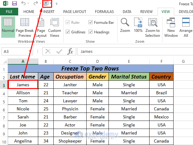8. Select Freeze Panes from the options.
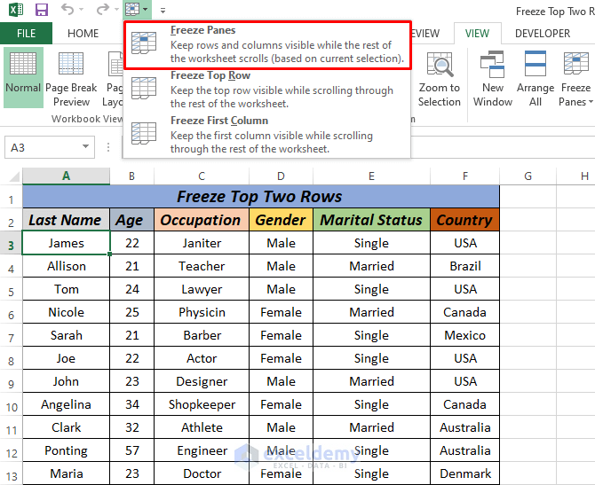9. The top two rows are frozen.

Related Content: How to Freeze 2 Columns in Excel

Things to Remember

Always click on the first cell in the row below the row or rows you want to freeze. For example, if you want to freeze the top two rows, you have to click on the first cell in the third row. If you select the second cell, you’ll also freeze the first column.

Practice Section

You can practice freezing the top rows with pretty much any sheet, but here’s a premade one for your convenience.

Download Practice Workbook

Related Articles

• How to Freeze First 3 Columns in Excel
• Unfreeze Rows in Excel
• How to Unfreeze Columns in Excel
• How to Freeze Random Selection in Excel
• How to Lock Cells in Excel When Scrolling
• How to Unlock Cells in Excel When Scrolling
• How to Lock Rows in Excel When Scrolling 

<< Go Back to Freeze Panes | Learn Excel