Often you need to generate random numbers or strings for specific purposes, especially in the case of statistical sampling. However, you have to freeze the random selection for further use. In this instructive session, I’ll show you 3 methods based on the 2 scenarios on how to freeze random selection in Excel.
Freeze Random Selection in Excel
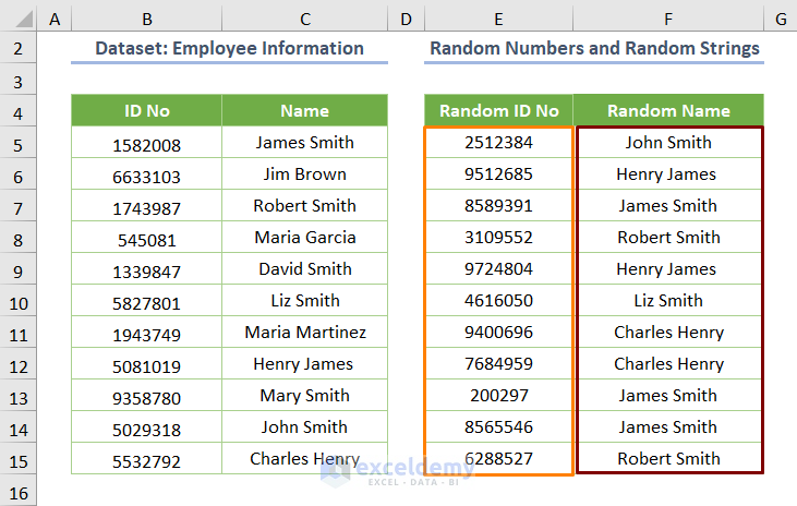
Let’s introduce today’s dataset where the Employee Information is given along with their ID No and Name. Besides, Random ID No and Random Name are displayed in columns E and F respectively.
So, you have to freeze either random numbers or random strings. Because these are continuously changing even if you click a single option in Excel. On the whole, you can utilize the following 3 methods to freeze random selection.
- Utilizing the Paste Options
- Dragging the selection holding right-clicking
- Changing the calculation options from Automatic to Manual
Now, I’m going to show you the application of these methods based on 2 different scenarios. The first scenario deals with the methods to freeze random numbers and the rest scenario addresses the methods to freeze random strings.
Let’s explore the methods.
Scenario 1: Methods to Freeze Random Numeric Selection
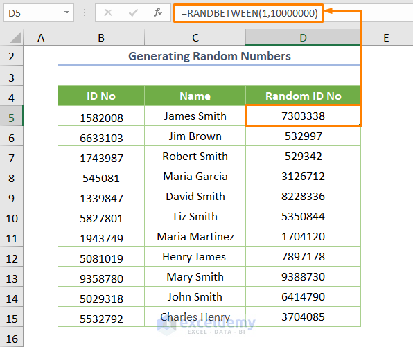
Let’s generate the random numbers using the RANDBETWEEN function before going to the methods of freezing. The function returns integer numbers between two given numbers.
For example, if you want to get the integer numbers between 1 and 10000000, you can use the formula below.
=RANDBETWEEN(1,10000000)
Here, 1 is the bottom argument and 10000000 is the top argument.
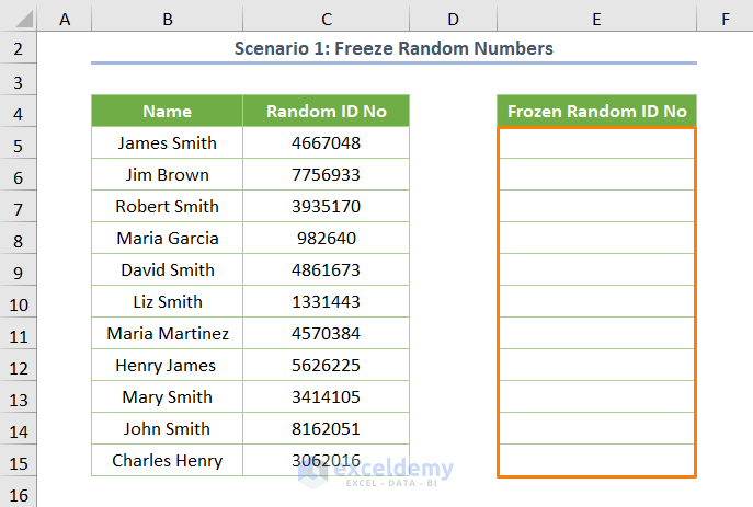
Now, you need to freeze the random numbers in the E5:E15 cell range.
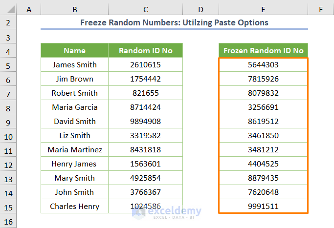
1. Utilizing Paste Options
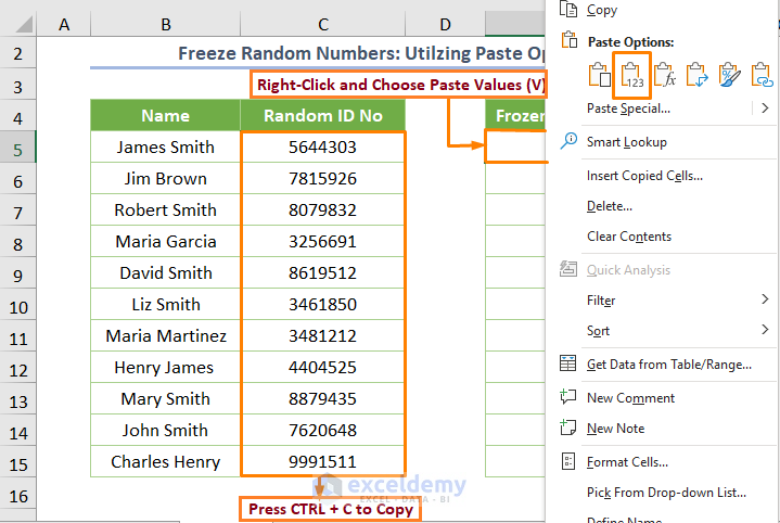
Luckily, you can freeze the random numbers utilizing the Paste Options feature in Excel. Please do the following task.
➜ Initially select the C5:C15 cell range and press CTRL + C to copy the random numbers.
➜ Later, go to the Context Menu by right-clicking (in the E5 cell) and choose the Values (V), one of the paste options (under the Paste Options feature).
Eventually, you’ll get the frozen random numbers in the E5:E15 cell range.
Read More: How to Freeze Top Row in Excel
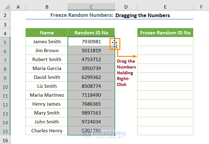
2. Dragging Numbers Holding Right-Click
Again, you can execute the same task by following this method.
➜ Select the random numbers first and then move your cursor over the border of the cell range.
➜ Then, you’ll see an icon of the move pointer as shown in the following image, and then drag the random numbers holding right-clicking (remember this, otherwise this method won’t work) to the E5:E15 cell range.
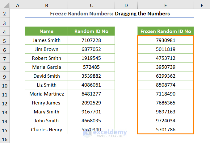
➜ Shortly, you’ll get some options after quitting right-clicking. Then, choose the Copy Here as Values Only option.
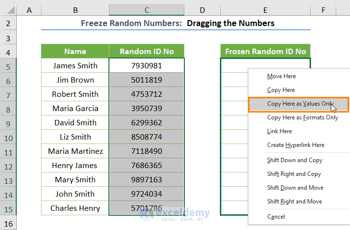
Eventually, you’ll get the frozen random numbers that won’t change.
Read More: How to Freeze Top Two Rows in Excel
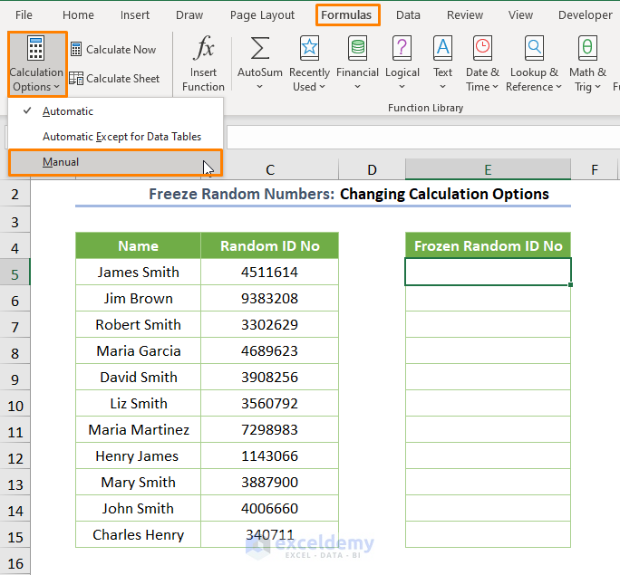
3. Changing Calculation Options from Automatic to Manual
The random numbers are changing incessantly because the calculation option is set as Automatic. So, if you change the option to Manual, the random numbers won’t change further. Let’s do it.
➜ Just go to the Formulas tab > click the drop-down list of the Calculation Options > choose the Manual option.
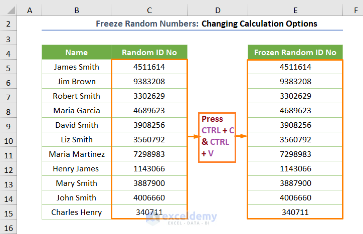
Now, if you copy (press CTRL + C) the random numbers and paste (press CTRL + V) them to another location, you’ll get the frozen random numbers. Certainly, the numbers won’t change.
Read More: How to Lock Cells in Excel When Scrolling
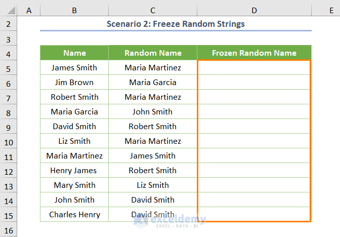
Scenario 2: Methods to Freeze Random Strings Selection
In this scenario, you’ll explore how to create random strings or texts and then the methods to freeze the random strings.
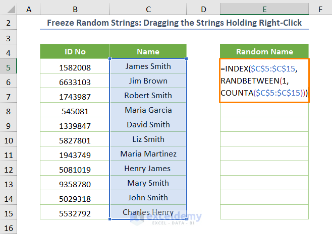
Let’s say, you want to generate a Random Name list in the E5:E15 cell range of the Name given in the C5:C15 cell range.
Just use the following formula in the E5 cell.
=INDEX($C$5:$C$15,RANDBETWEEN(1,COUNTA($C$5:$C$15)))
Here, C5:C15 is the cell range representing Name.
⧬ In the above formula, the COUNTA function counts the row number of the C5:C15 cell range. Subsequently, the RNADBETWEEN function generates random numbers from the 1 to the found row number in the previous output. Lastly, the INDEX function returns the random name based on the random number generated by the RNADBETWEEN function.
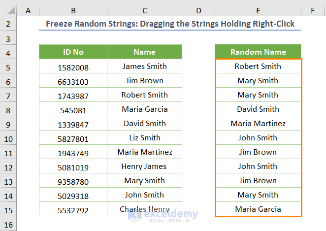
After pressing ENTER and using the Fill Handle tool, you’ll get the Random Name list.
Now, come to the main topic! You have to freeze the random strings.
Read More: How to Unlock Cells in Excel When Scrolling
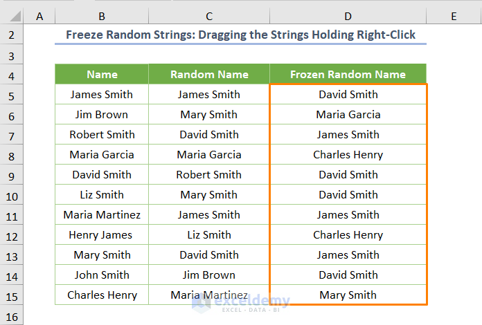
1. Dragging Strings Holding Right-Click
As shown in Method 2 of Scenario 1, you can easily drag the strings to the D5:D15 cells holding right-click.
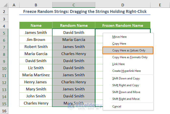
Therefore, you’ll get the frozen random name after choosing the Copy Here as Values Only option.
Read More: How to Lock Rows in Excel When Scrolling
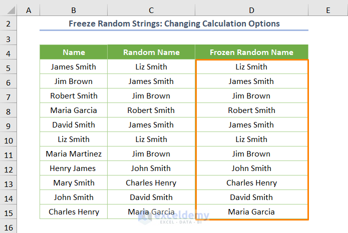
2. Changing Calculation Options
Similarly, you may change the calculation option from Automatic to Manual as discussed in Method 3 of Scenario 1.
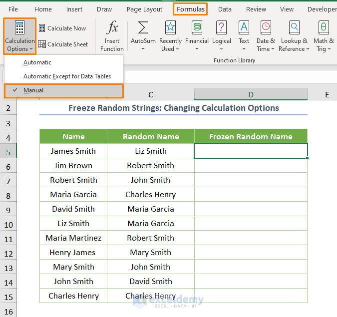
After copy-pasting the random strings from column C to D, you’ll get the following output.
Read More: How to Freeze Top 3 Rows in Excel
Download Practice Workbook
Conclusion
That’s the end of today’s session. Surely, I believe from now you can freeze random selection in Excel effectively. If you find this article fruitful, don’t forget to share it in your community. Anyway, if you have any queries or recommendations, please share them in the comments section below.
Related Articles
- How to Freeze Columns in Excel
- How to Freeze 2 Columns in Excel
- How to Freeze First 3 Columns in Excel
- Unfreeze Rows in Excel
- How to Unfreeze Columns in Excel
<< Go Back to Freeze Panes | Learn Excel
Get FREE Advanced Excel Exercises with Solutions!
