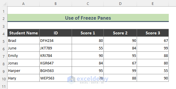
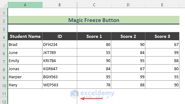
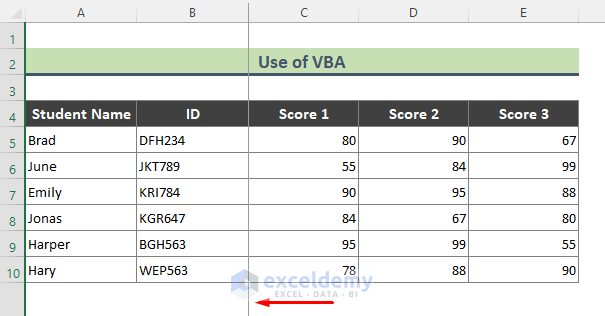
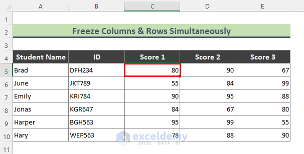
We have a dataset containing several students’ Names, IDs, Test Scores, etc. As the dataset contains scores of several tests, scrolling right to the worksheet hides columns A and B. We will freeze columns A and B so that columns having Student Name and ID are visible all the time.
Method 1 – Freeze 2 Columns Using the Freeze Panes Option in Excel
Steps:
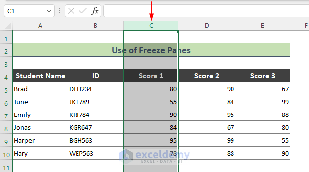
- Select the column that is next to the first 2 columns. We selected column C.
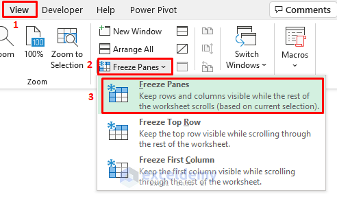
- From the Excel Ribbon, go to View, then to Freeze Panes, and click Freeze Panes.
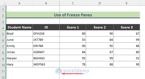
- A gray line appears after column B, and the two columns before that line are frozen.
Note:
You can freeze the first two columns by using the keyboard shortcut Alt + W + F + F (pressing one by one).
Read More: How to Freeze First 3 Columns in Excel
Method 2 – Apply the Excel Split Option to Freeze 2 Columns
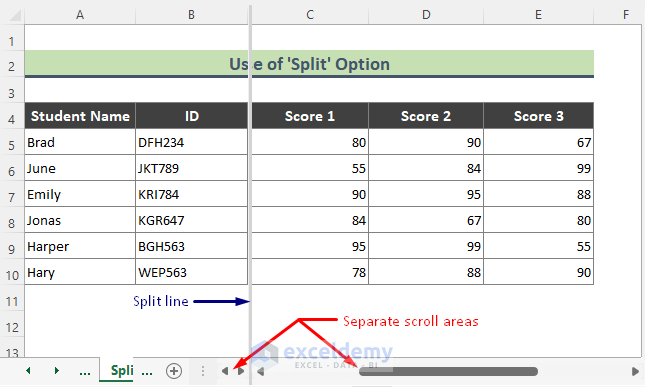
By applying Split after the first 2 columns, it divides the Excel worksheet areas into two separate areas. In both of these areas, you can scroll the dataset right or left.
Steps:
- Select column C.
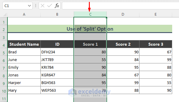
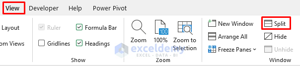
- Go to View and select Split.
- The corresponding worksheet containing the dataset is split after the first 2 columns. You will see separate scroll areas, too.
Read More: How to Freeze Columns in Excel
Method 3 – Lock 2 Columns Using the Magic Freeze Button in Excel
Steps:
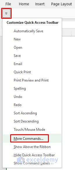
- Click on the Customize Quick Access Toolbar icon and select the More Commands option.
- The Excel Options window will appear.
- Choose the Freeze Panes command under Popular Commands, click on the Add button, and press OK.
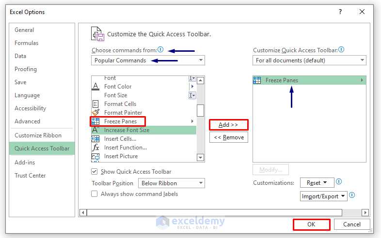
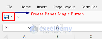
- The Magic Freeze button is added to the Quick Access Toolbar.
- Similar to Method 1, select column C and click Freeze Panes from the Magic Freeze button.
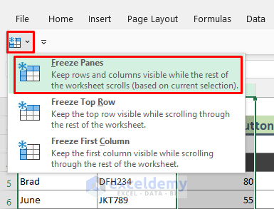
- The gray line appears, and the first two columns are frozen.
Read More: How to Unfreeze Columns in Excel
Method 4 – Apply VBA to Freeze 2 Columns in Excel
Steps:
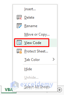
- Go to the worksheet where you want to freeze 2 columns.
- Right-click on the sheet name and click on the View Code option to bring up the VBA window.
- Copy the below code in the Module. We have written Columns (C:C) in the code, as we want to freeze columns A and B. Change the code as you require.
Sub Freeze2Columns()

    Columns("C:C").Select
    ActiveWindow.FreezePanes = True

End Sub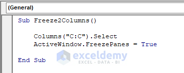
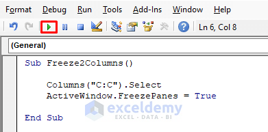
- Run the code by pressing the F5 key or clicking on the Run icon (see the screenshot).
- The first two columns of the worksheet are frozen.
Read More: How to Freeze Top Row in Excel
Method 5 – Freeze Rows and 2 Columns Simultaneously
Steps:
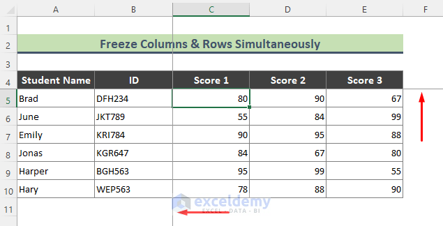
- Click Cell C5 (Cell right to the column and below to the row you want to freeze).
- Go to View, then to Freeze Panes, and select Freeze Panes.
- Two grey lines appear, which indicate that the first 2 columns and the top 4 rows are frozen.
Read More: How to Freeze Top Two Rows in Excel
Unfreeze Columns in Excel
Steps:
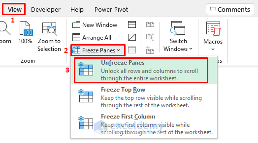
- Go to the worksheet where columns are frozen.
- Go to View, select Freeze Panes, and click on Unfreeze Panes.
Note:
You can apply this keyboard shortcut to unfreeze columns: Alt + W + F + F
Related Content: How to Freeze Top 3 Rows in Excel
Download the Practice Workbook
Related Articles
- Unfreeze Rows in Excel
- How to Freeze Random Selection in Excel
- How to Lock Cells in Excel When Scrolling
- How to Unlock Cells in Excel When Scrolling
- How to Lock Rows in Excel When Scrolling
<< Go Back to Freeze Panes | Learn Excel
Get FREE Advanced Excel Exercises with Solutions!
