How to Freeze Panes with VBA in Excel (5 Ways)

Sub Freeze_Panes_Row_and_Column()

Range("C4").Select

ActiveWindow.FreezePanes = True

End Sub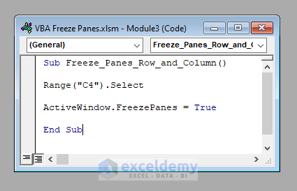

Method 1 – Freezing a Row with VBA in Excel

Steps:

• Select the row below the row to be frozen (Row 4 in this example).
• Apply the Freeze Panes command.
• So the VBA code will be:

⧭ VBA Code:

Sub Freeze_Panes_Only_Row()

Range("C4").EntireRow.Select

ActiveWindow.FreezePanes = True

Range("C4").Select

End Sub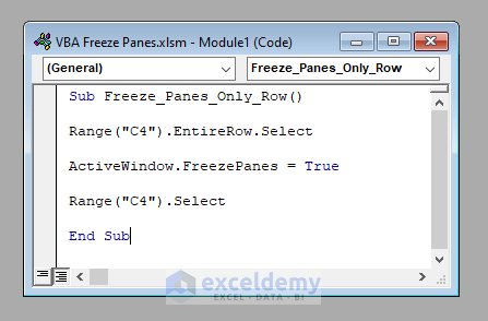

• Run this code. The active worksheet is frozen up to row 3.

⧭ Notes:

• Here, we’ve used cell C4 to select any cell in row 4 of the worksheet. You can select it according to your needs.
• The last line of the code Range(“C4”).Select is for deselecting the entire row 4 (Deselecting any selection means selecting a new selection, as in Excel, something must remain selected). You can omit this line if you want.

Read More: Keyboard Shortcut to Freeze Panes in Excel

Method 2 – Freezing a Column with VBA in Excel

Steps:

• Select the entire column right to the column to be frozen (Column C in this example).
• Apply the Freeze Panes command.
• The VBA code will be:

Sub Freeze_Panes_Only_Column()

Range("C4").EntireColumn.Select

ActiveWindow.FreezePanes = True

Range("C4").Select

End Sub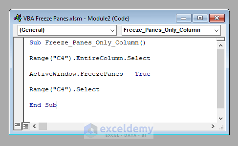

• Run this code. The active worksheet is frozen up to column C.

⧭ Notes:

• Here we’ve used cell C4 to select any cell of column C of the worksheet. You select it according to your needs.
• The last line of the code Range(“C4”).Select is for deselecting the entire column C (Deselecting any selection means selecting a new selection, as in Excel, something must remain selected). You can omit this line if you want.

Read More: How to Apply Custom Freeze Panes in Excel

Method 3 – Freezing both a Row and a Column with VBA in Excel

Steps:

• Select a cell below the row to be frozen and right to the column to be frozen (Cell C4 in this example).
• Apply the Freeze Panes command.
• The VBA code will be:

Sub Freeze_Panes_Row_and_Column()

Range("C4").Select

ActiveWindow.FreezePanes = True

End Sub

• Run this code. The active worksheet is frozen up to row 3 and column C.

⧭ Notes:

• Here, we’ve used cell C4 to select a cell below row 3 and right in column B. That’s cell C4. You select it according to your needs.

Read More: How to Freeze Rows and Columns at the Same Time in Excel 

Method 4 – Developing a Userform to Freeze Panes with VBA in Excel

Steps:

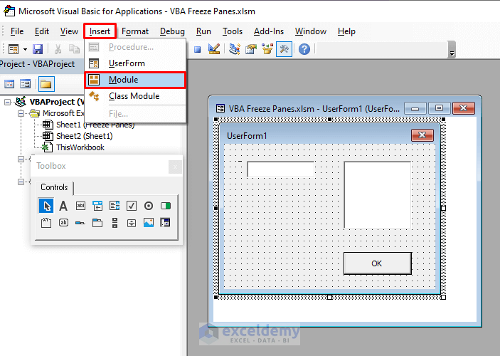
• Press ALT+F11 to open the Visual Basic
• Go to Insert > UserForm to insert a new Userform.

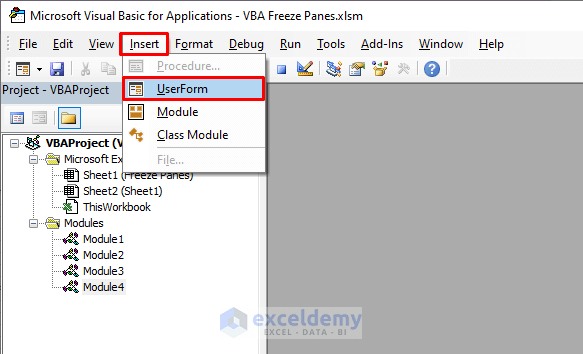
• A new UserForm called UserForm1 will be created in the VBA
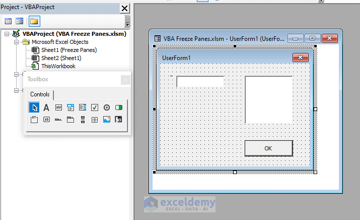
• On the left of the UserForm, you’ll get a ToolBox called Control. Hover your mouse on the toolbox and search for a TextBox (TextBox1). After finding one, drag it over the top of the UserForm.
• Drag a ListBox (ListBox1) right to the Textbox and a CommandButton (Commandbutton1) to the bottom right corner of the UserForm.
• Change the display of the CommandButton to OK.

Your UserForm should now look like this:

• Insert a Module (Insert > Module) from the VBA toolbox.

• Enter the following VBA code in the Module:

Sub Run_UserForm()

UserForm1.Caption = "Freeze Panes"

UserForm1.TextBox1.Text = Selection.Address
UserForm1.TextBox1.BorderStyle = fmBorderStyleSingle

UserForm1.ListBox1.BorderStyle = fmBorderStyleSingle
UserForm1.ListBox1.ListStyle = fmListStyleOption

UserForm1.ListBox1.AddItem "1. Freeze Row"
UserForm1.ListBox1.AddItem "2. Freeze Column"
UserForm1.ListBox1.AddItem "3. Freeze Both Row and Column"

Load UserForm1
UserForm1.Show

End Sub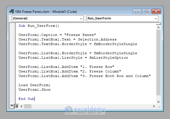

• Double-click on the CommandButton, which is displayed as OK. A Private Sub called CommandButton1_Click will open.
• Enter the following code:

    If UserForm1.ListBox1.Selected(0) = True Then
        Set Rng = Selection
        Rng.EntireRow.Select
        ActiveWindow.FreezePanes = True
        Rng.Select

    ElseIf UserForm1.ListBox1.Selected(1) = True Then
        Set Rng = Selection
        Rng.EntireColumn.Select
        ActiveWindow.FreezePanes = True
        Rng.Select

    ElseIf UserForm1.ListBox1.Selected(2) = True Then
        ActiveWindow.FreezePanes = True

    Else
        MsgBox "Select At Least One. ", vbExclamation

    End If

    Unload UserForm1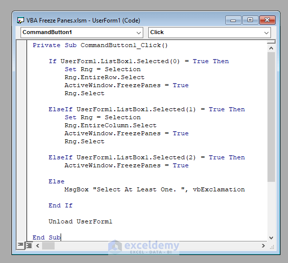

• Double-click on TextBox1. A Private Sub called TextBox1_Change will open.
• Enter the following code:

Private Sub TextBox1_Change()

On Error GoTo Message

Range(TextBox1.Text).Select

Message:
    Note = 5

End Sub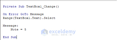

Your UserForm is now ready to use.

• Select the cell below the row to be frozen and right to the column to be frozen (Cell C4 here).
• Run the Macro called Run_UserForm.

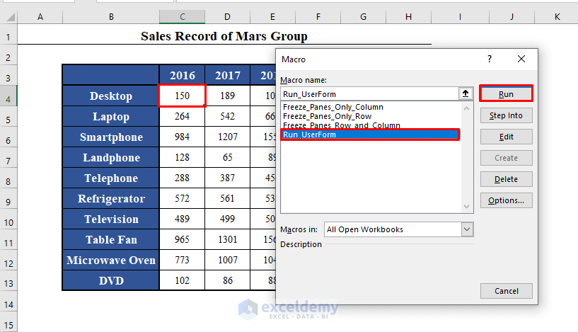
• The UserForm will be loaded. You’ll find the address of the selected cell (C4) in the TextBox. If you want, you can change this.
• Select any one of the three options available in the ListBox. Here, I want to freeze both row and column, so I’ve selected Freeze Both Row and Column.
• Click OK.

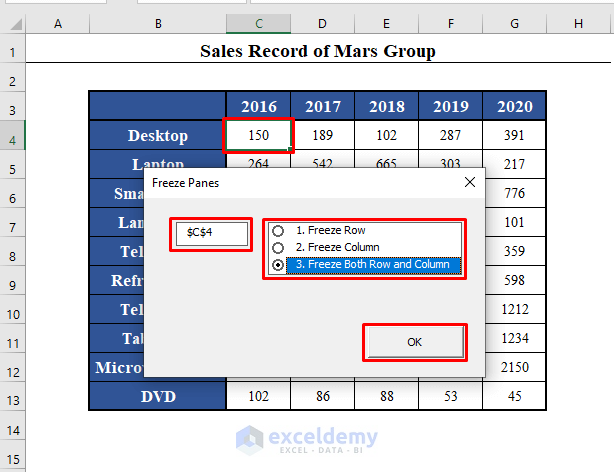
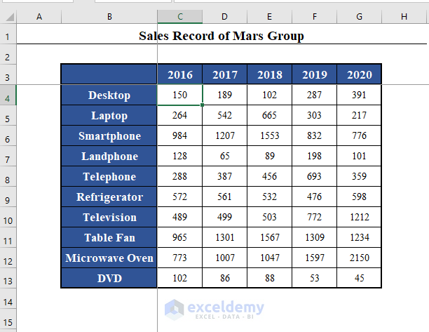
The worksheet is frozen. (It is frozen up to row 3 and column B here.)

Related Content: Excel Freeze Panes Not Working

Method 5 – An alternative to the Freeze Panes in Excel: Split the Window with VBA

Steps:

You can ActiveWindow.SplitRow or ActiveWindow.SplitColumn in VBA to split the worksheet row-wise or column-wise.

• To split the worksheet from row 3, use:

ActiveWindow.SplitRow = 3

• To split the worksheet from column B, use:

ActiveWindow.SplitColumn = 2

⧭ VBA Code:

Sub Split_Window()

ActiveWindow.SplitRow = 3

ActiveWindow.SplitColumn = 2

End Sub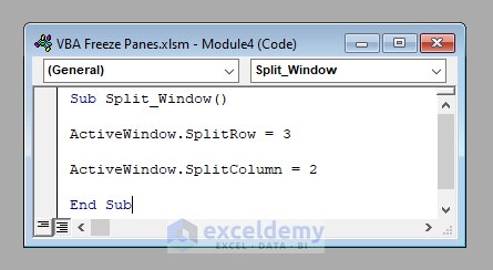

• Run the code, It’ll split the active worksheet from row 3 and column B.

Related Content: How to Unfreeze Rows and Columns in Excel

Things to Remember

• Before applying Freeze Panes in Excel, you must Unfreeze all the Freeze Panes already applied. Otherwise, the Freeze Panes command won’t work.
• The Freeze Panes command won’t work through the merged cells. So, unmerge them before applying the Freeze Panes command if there is any.

Download the Practice Workbook

Download this workbook to practice.

Conclusion

So these are the methods to use Freeze Panes with VBA in Excel. I’ve tried to discuss all possible ways to apply Freeze Panes over a worksheet in Excel. Do you have any questions? Feel free to ask us.

Related Articles

• How to Freeze Multiple Panes in Excel
• How to Freeze Top Row and First Column in Excel

<< Go Back to Freeze Panes | Learn Excel