How to Use The Keyboard Shortcut to Freeze Panes in Excel (3 Methods)

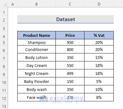
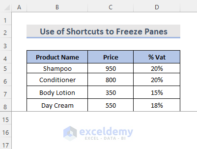
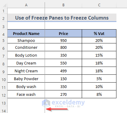
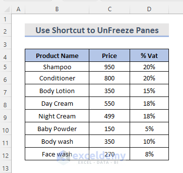
The dataset includes the Product Name, the Price, and the product’s percentage of value-added tax (VAT).

Method 1 – Shortcut to Freeze Both Rows and Columns

STEPS:

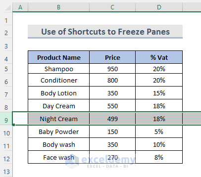
• Select the cell row or column (i.e., row 9).
• Click on row 9, or on any cell in row 9, and press Shift + Spacebar, to select the whole row.

• Press  Alt + W + F, at the same time. The Freeze Panes option will open.
• Press F to Freeze Panes.

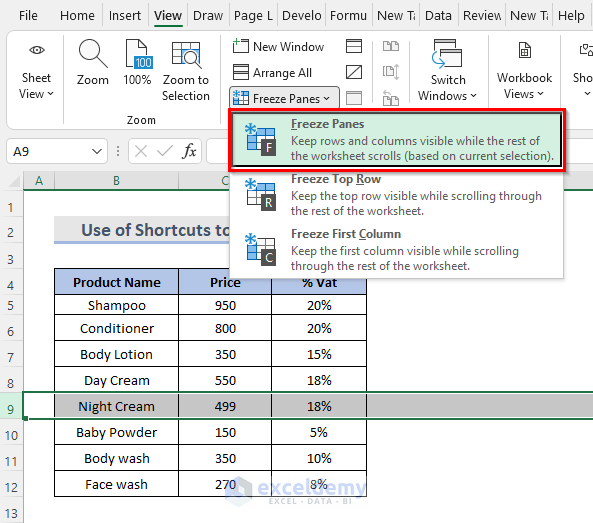
• Press Alt + W + F + F to freeze the panes.
• A gray line will appear directly below the frozen rows.

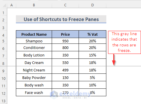
• If we scroll down, the frozen rows will still be visible.

Read More: How to Freeze Top Row and First Column in Excel

Method 2 – Shortcut to Freeze Top Rows

STEPS:

• Press Alt + W + F. The Freeze Panes drop-down menu bar will open.
  

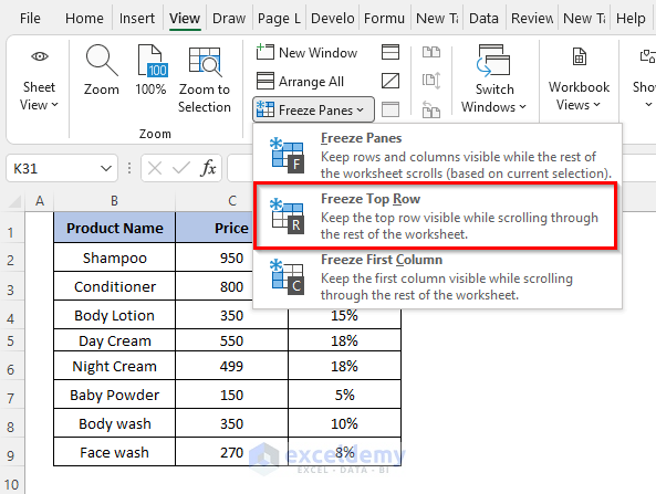
• Press R to lock the top rows.
• A gray line appears. The headers are now locked.

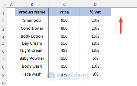
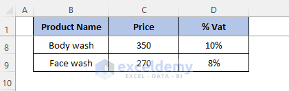
• If we scroll down, the headers will remain in the same place.

Read More: How to Freeze Multiple Panes in Excel

Method 3 – Freeze the First Column with the Keyboard Shortcut

STEPS:

• Use the keyboard shortcut Alt + W + F to open the Freeze Panes menu bar.

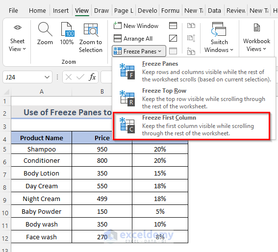
• To lock the first column, press C. This will freeze the first column of our worksheet.

• If we scroll left or right, the first column will remain in the same place.

Read More: How to Freeze Rows and Columns at the Same Time in Excel 

Shortcut of Unfreeze Panes in Excel

STEPS:

• Press Alt + W + F, to open the Freeze Panes menu bar.

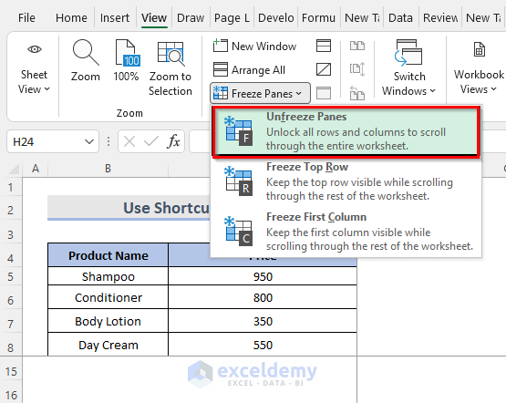
• Press F to unfreeze the panes.

Download the Practice Workbook

Related Articles

• How to Unfreeze Rows and Columns in Excel
• How to Apply Custom Freeze Panes in Excel
• Excel Freeze Panes Not Working
• How to Freeze Panes with VBA in Excel 

<< Go Back to Freeze Panes | Learn Excel