In Excel, we use the Freeze Panes feature to lock or fix specific rows or columns in your worksheet so that they remain visible as we scroll through the rest of the data. This can make comparing and analyzing data easier, especially if we have a huge data table.
In this Excel tutorial, you will learn how to
– freeze the top row
– freeze the first column
– lock multiple rows and columns
– add the Freeze Panes button in the Quick Access toolbar
– unfreeze panes
– and some alternatives to freezing panes in Excel
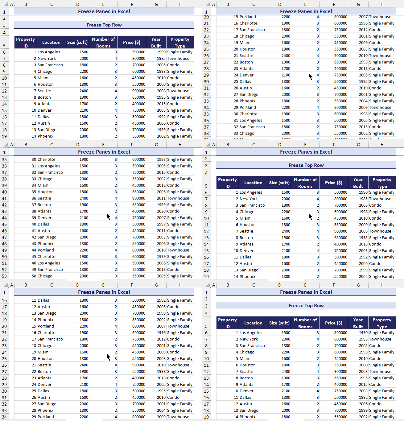
Consider the following dataset. It contains 60 rows and 11 columns. Here, I have fixed the top row to keep this row visible while scrolling through.
⏷Purpose of Freezing Panes in Excel
⏷Freeze Row Panes
⏵Top Row
⏵Top Two Rows
⏵Multiple Rows at Once
⏷Freeze Column Panes
⏵Left Column
⏵First Two Columns from the Left
⏵Multiple Columns at Once
⏷Freeze Multiple Rows and Columns
⏷Keyboard Shortcuts to Freeze Panes
⏷VBA Code to Freeze Multiple Rows and Columns at Once
⏷Add Magic Freeze Button
⏷Navigation with Freeze Panes
⏷Unfreeze Panes in Excel
⏷Alternatives to Freeze Panes in Excel
⏵Use Split Option from the View Tab
⏵Open a New Window for the Current Workbook
⏵Insert Table to Lock the First Row
⏷Reasons behind Freeze Panes Not Working
What Is the Purpose of Freezing Panes in Excel?
The purpose of freezing panes in Excel is –
- to keep some rows or columns visible while scrolling through the rest of the data in a worksheet
- to prevent repetition throughout a large dataset
- to keep the column headers to understand which data represents what
- compare different sections of data.
How to Freeze Row Panes in Excel
Using the Freeze Panes feature, you can easily freeze the top row or even multiple rows in Excel.
1. Freeze Top Row
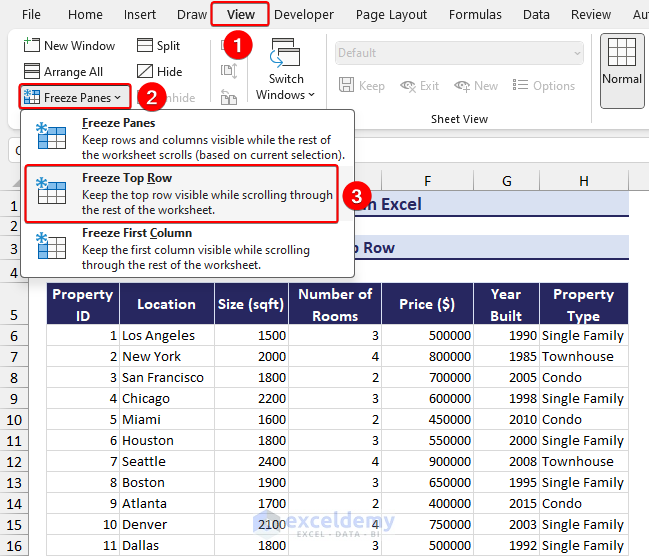
To freeze the top row, I will use the Freeze Top Row option to keep the column headers visible while scrolling.
- Click on the View tab >> Select the Freeze Panes option. Then, choose the Freeze Top Row option.
- As a result, you can see the first row has been frozen. If you scroll down, the top row is still visible.
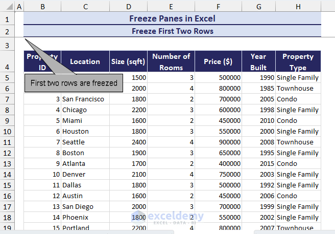
2. Freeze Top Two Rows
In this method, I want to freeze the first two rows. When I scroll through the dataset, the first two rows should be visible.
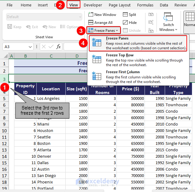
- First, click the row bar of the 3rd row to select the entire row.
- Now, go to the View tab >> click the Freeze Panes dropdown >> select Freeze Panes option.
- After clicking the Freeze Panes option, the top two rows are now fixed.
3. Freeze Multiple Rows at Once
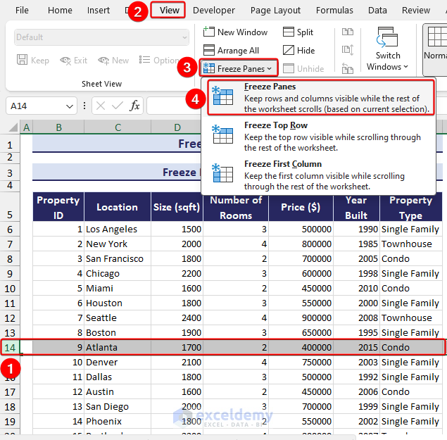
Suppose, we want to compare all data with the data of the first 13 rows. Therefore, I need to keep the first 13 rows visible when I scroll down. To do this, you can apply the following steps.
- First, select the 14th row.
- Then go to the View tab >> click on the Freeze Panes dropdown >> select the Freeze Panes option.
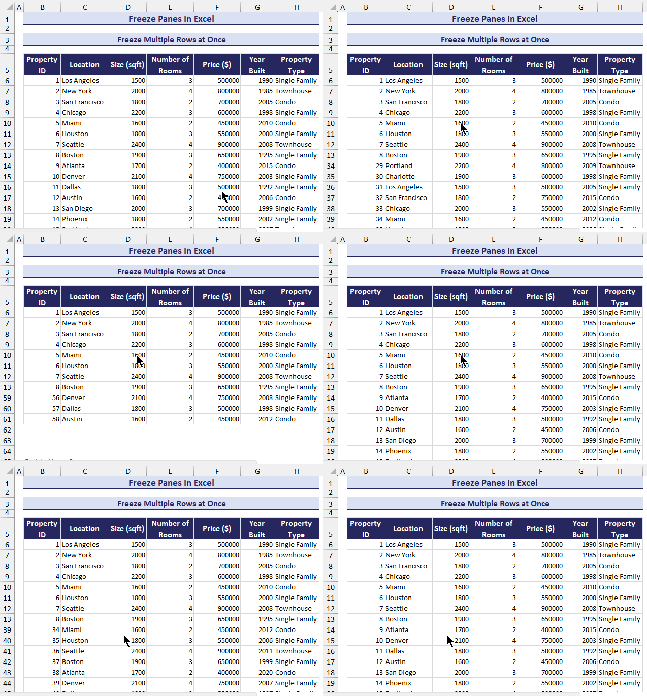
- As a result, the first 13 rows of the dataset are now frozen.
How to Freeze Column Panes in Excel
We can use the Freeze Panes option to freeze columns as well. It offers to freeze single or multiple columns at once.
1. Freeze Left Column
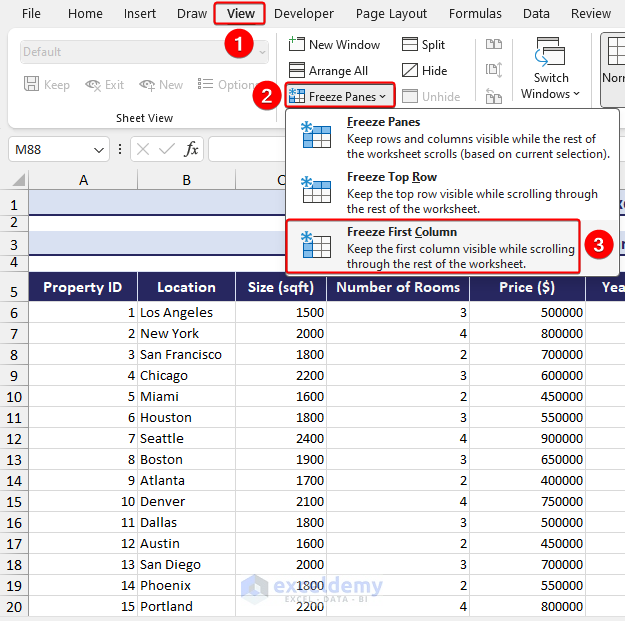
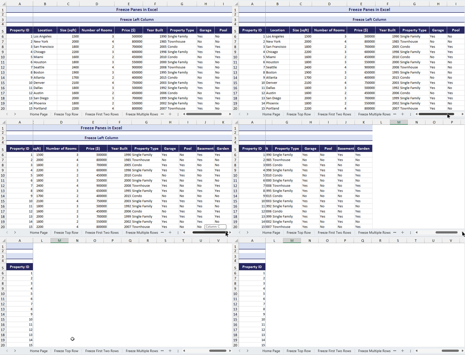
Here, I’ve data in multiple columns and want to compare the values according to the first column. I can freeze the first column using the Freeze First Column option.
- First, click on the View tab >> Select the Freeze Panes dropdown >> Select the Freeze First Column option.
- As a result, the first column has been frozen. If you scroll horizontally to the right, the first column will not go away.
2. Freeze the First two Columns from the Left
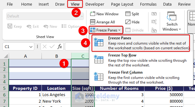
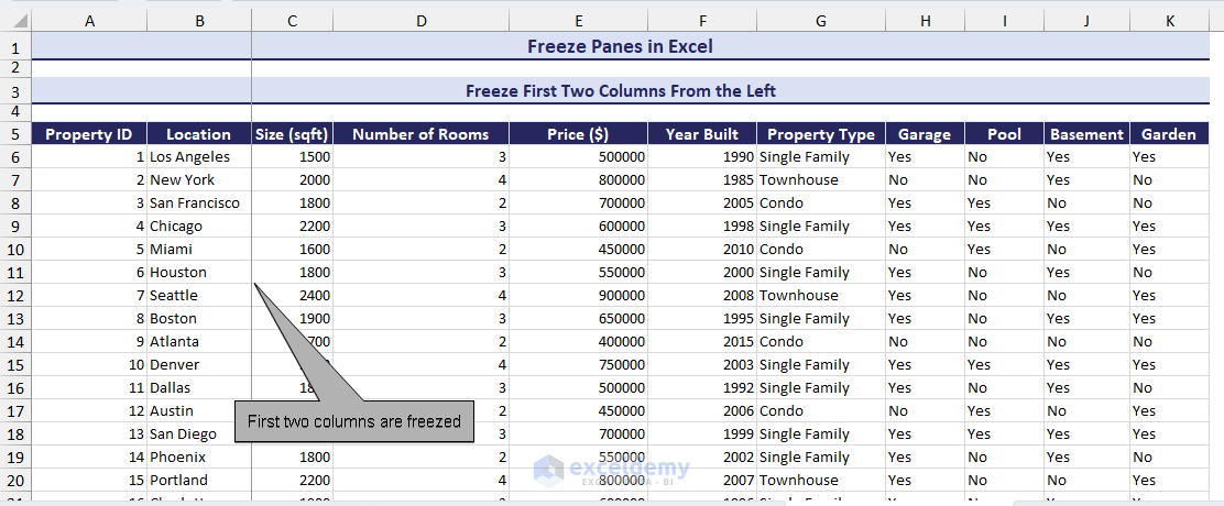
We want to keep the first two columns visible while scrolling. We will lock the first two columns with the help of Freeze Panes.
- To begin, select the entire C column.
- Go to the View tab >> click the Freeze Panes dropdown >> select Freeze Panes option.
- Therefore, you’ve frozen the first two columns like in the image below.
3. Freeze Multiple Columns at Once
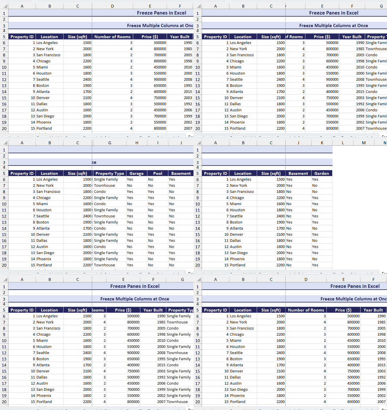
We can freeze multiple columns using the Freeze Panes option to ensure that the data remains visible. For this example, we will freeze the first 3 columns
- First, select the fourth column.
- Then go to the View tab >> click the Freeze Panes dropdown >> select Freeze Panes option.
- The A, B, and C columns will have been frozen. You can scroll to the right, keeping the first three columns visible.
How to Freeze Multiple Rows and Columns in Excel
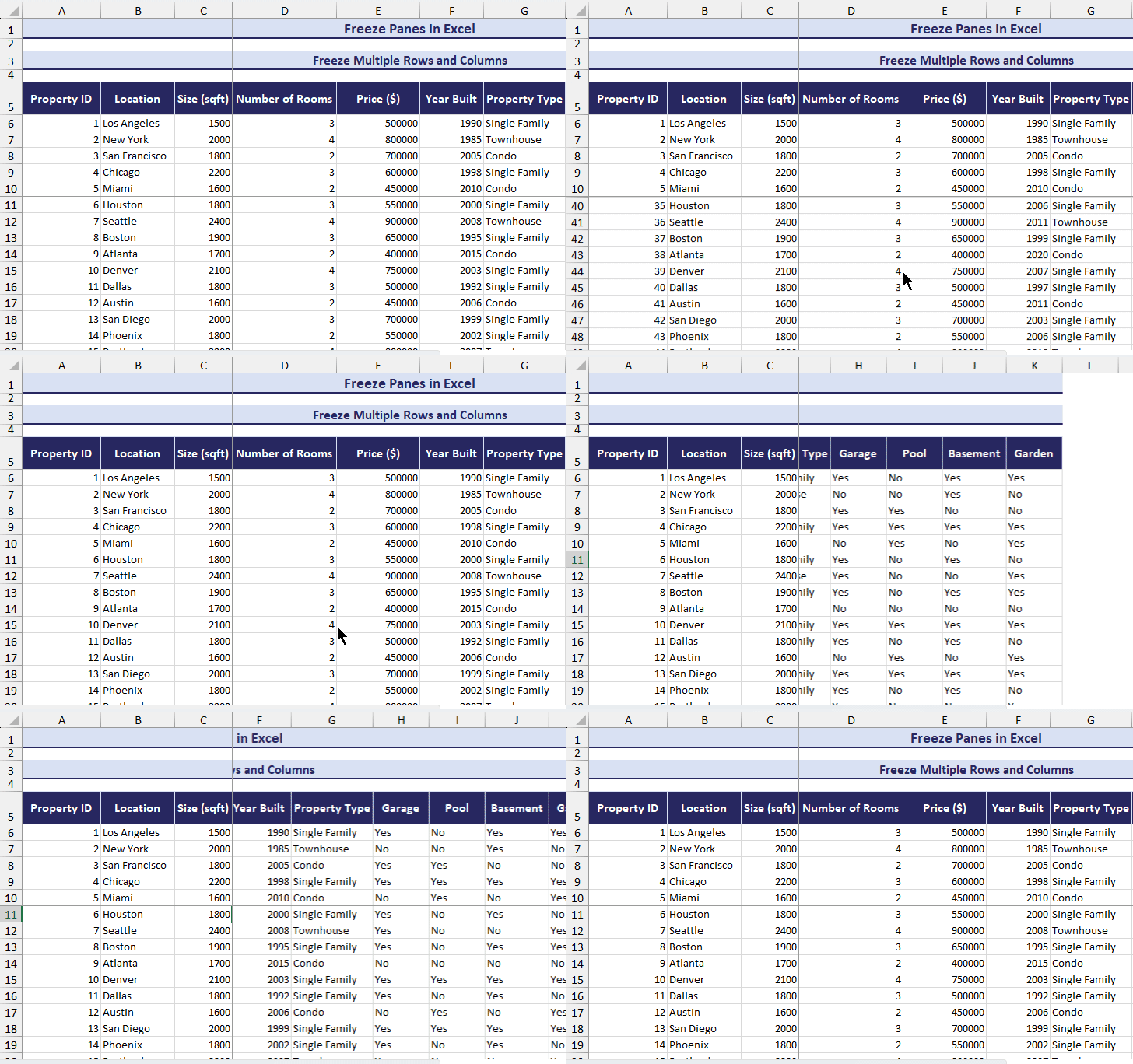
You can use the Freeze Panes option to freeze multiple rows and columns and keep them visible while scrolling both horizontally and vertically.
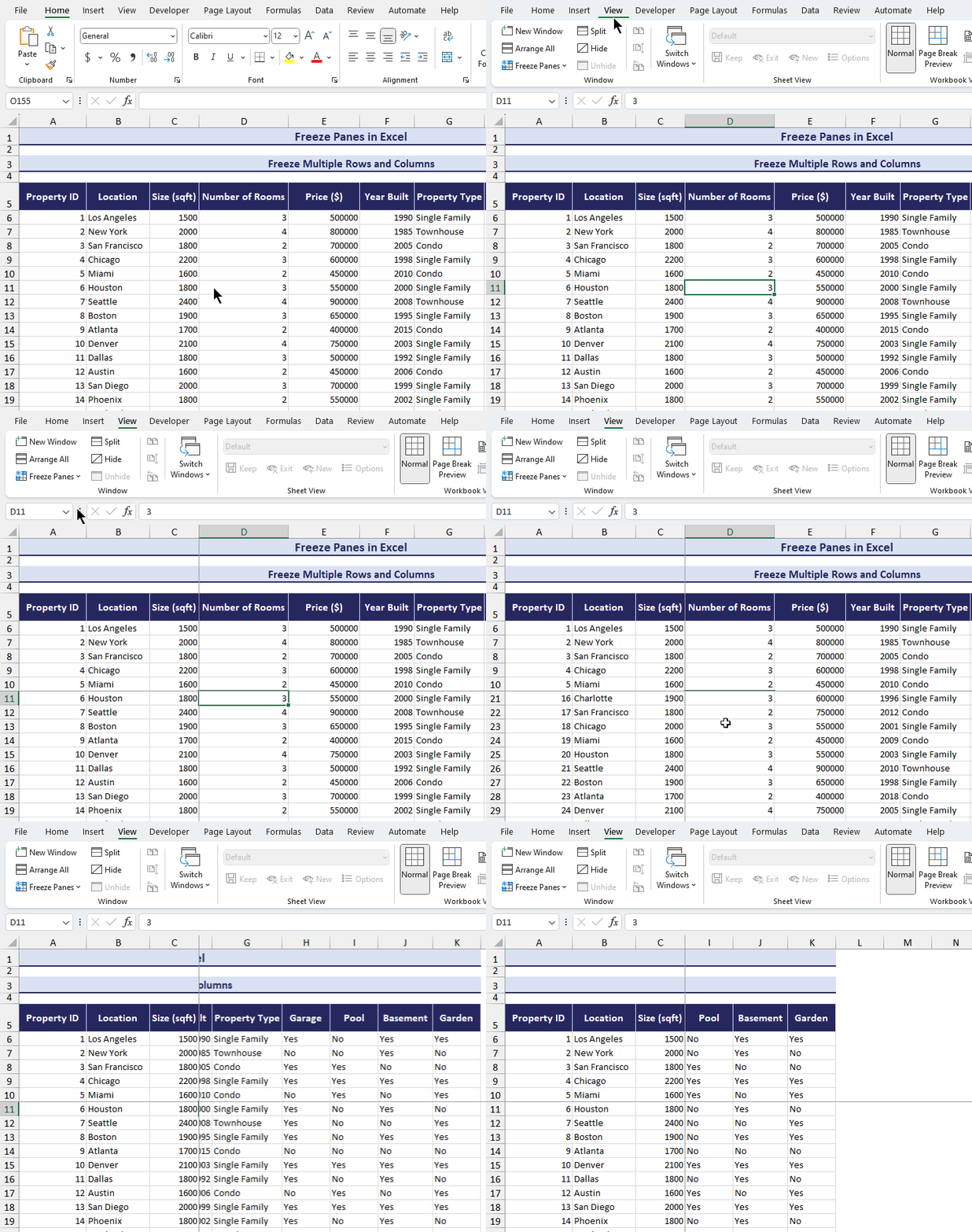
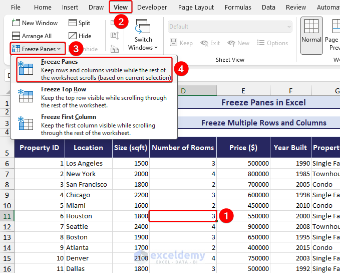
- First, select the cell that is located immediately below and to the right of the rows and columns you want to freeze. Here I have selected the D11 cell.
- Then click on the View tab >> Freeze Panes dropdown menu >> Select the Freeze Panes option.
- You can see that multiple rows and columns are frozen. Here, the first 10 rows and the first 4 columns will always be visible while scrolling.
Keyboard Shortcuts to Freeze Panes in Excel
The available keyboard shortcuts to freeze panes.
Shortcuts | What It Does |
---|---|
Alt+W+F+R | Freeze Top Row |
Alt+W+F+C | Freeze First Column |
Alt+W+F+F | Freeze Top Row and First Column (Freeze Panes) |
Alt+W+U | Unfreeze Panes |
Using the keyboard shortcuts to freeze panes helps to do the task quickly. The best part is you don’t have to navigate through various menus and options using the mouse.
How to Apply VBA to Freeze Multiple Rows and Columns at Once
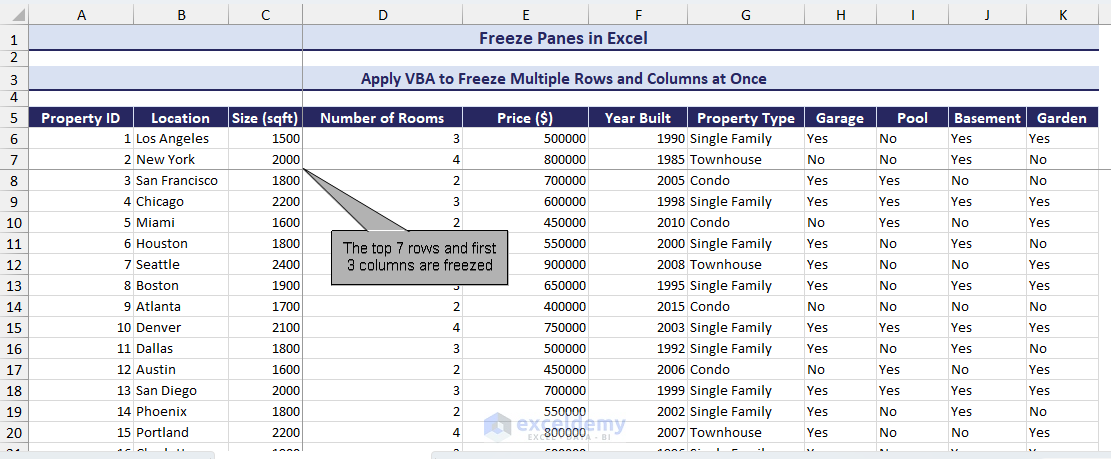
You can automate freezing panes in Excel by using VBA code. When we are working with numerous worksheets, it is smarter to use VBA code to freeze panes. In this method, we will use VBA to freeze the first seven rows and three columns of an Excel sheet.
- Click on the Developer tab >> you will notice the Visual Basic option in the Code section.
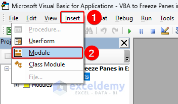
- After clicking on Visual Basic, Excel will lead you to the Visual Basic Editor Now, click Insert and select the Module option.
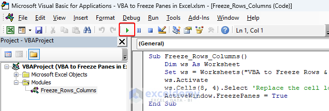
- Now, copy this code in Module1.
Sub Freeze_Rows_Columns()
Dim ws As Worksheet
Set ws = Worksheets("Using_VBA") ' Replace with your sheet name
ws.Activate
ws.Cells(9, 5).Select 'Replace the cell location
ActiveWindow.FreezePanes = True
End Sub
- Then, run this code by pressing the F5 key or clicking on the Run button.
- Running the code will freeze the first 7 rows and 3 columns as shown in the image below.
Code Breakdown
- Dim ws As Worksheet: Declares a variable named “ws” of type “Worksheet”. This variable will be used to refer to the worksheet.
- Set ws = Worksheets(“Using_VBA”): Assigns the worksheet named “Using_VBA” to the “ws” variable. Replace “Using_VBA” with the name of your target worksheet.
- Activate: Activates the worksheet referred to by the “ws” variable.
- Cells(8, 4).Select: Select the cell located in row 8 and column 5 in the active worksheet. This cell will be the point where the frozen panes are applied. Replace these values with the row and column numbers of the cell you want to use.
- FreezePanes = True: Sets the “FreezePanes” property of the active window to “True“, which freezes the rows and columns above and to the left of the selected cell. As a result, the selected cell becomes the upper-left corner of the visible area as you scroll through the sheet.
How to Add Freeze Panes (Magic Freeze Button) on the Excel Quick Access Toolbar
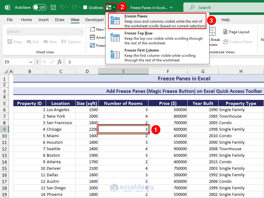
You can use the Magic Freeze Button to freeze or unfreeze panes with just one click.
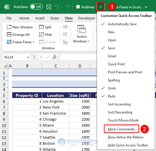
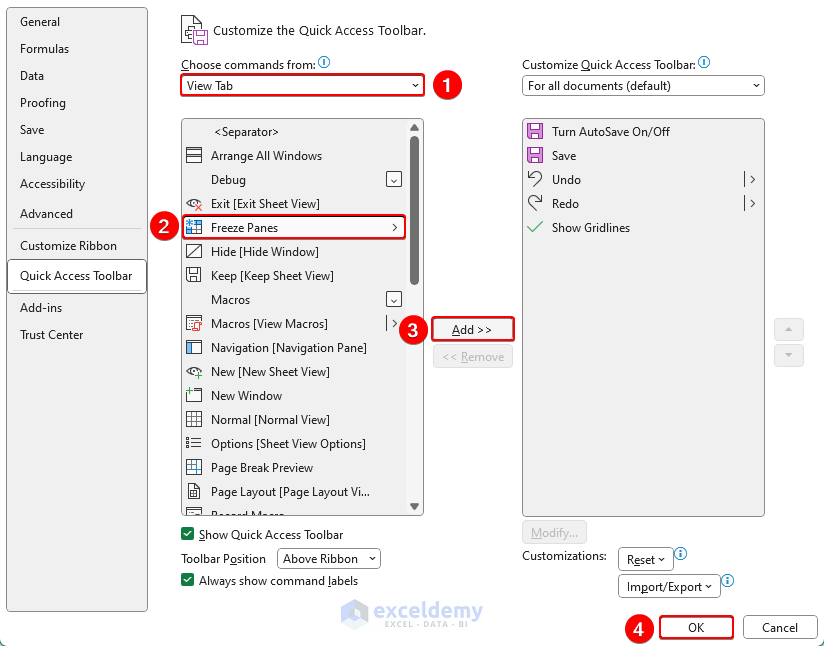
- First, click on the Customize Quick Access Toolbar (down arrow) button at the top of the worksheet, and select More Commands from the options.
- In Choose commands from, select View Tab from the dropdown.
- Select the Freeze Panes command >> click the Add button >> click OK.
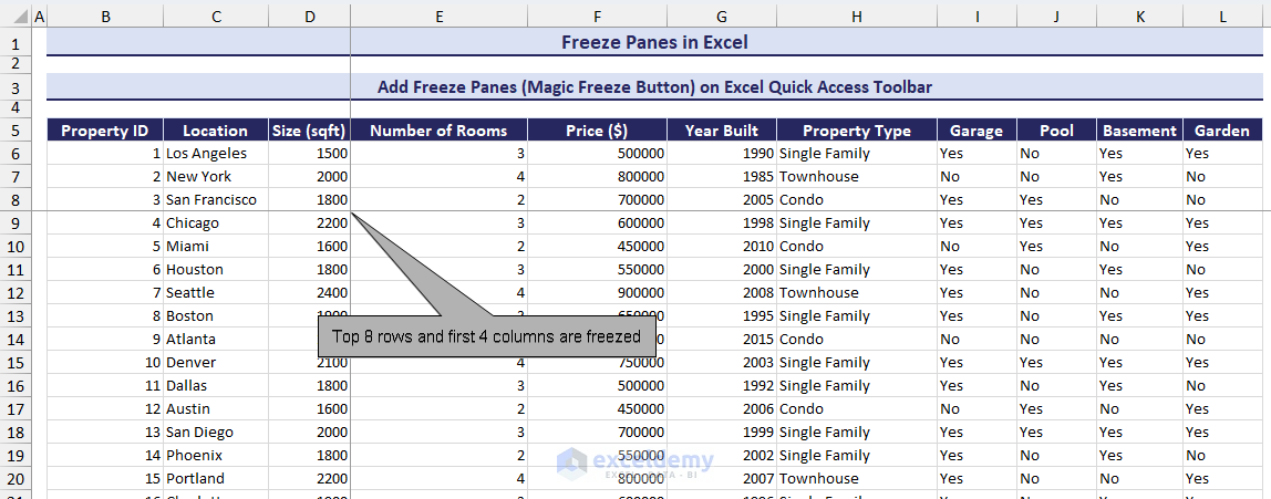
- You can see the Magic Freeze Button at the top of the toolbar. Now you can freeze/unfreeze panes just by selecting a cell and then clicking on the Freeze Panes option in the Magic Button.
- The result will be like the regular freezing rows and columns as in the image below.
Navigation with Freeze Panes in Excel
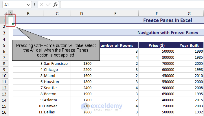
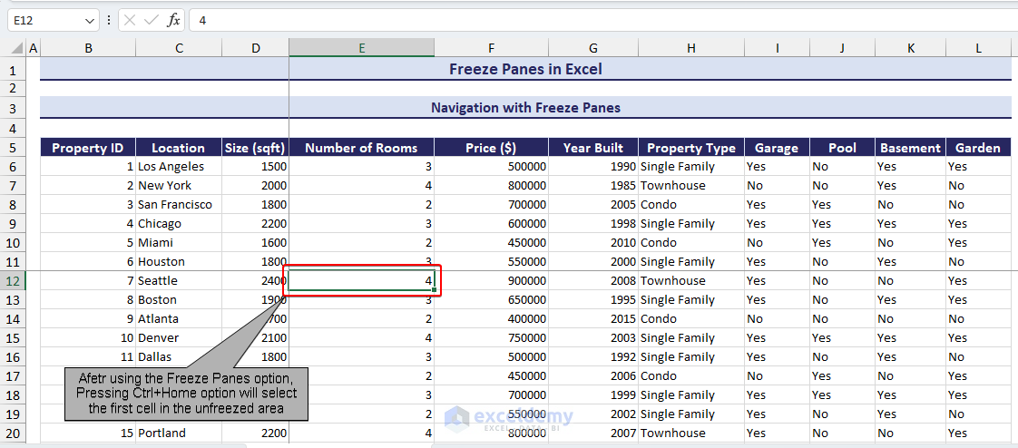
Using the Ctrl+Home keyboard shortcut, we can navigate to the “A1” cell when there are no freezed panes.
After freezing panes using the Freeze Panes feature in Excel, by pressing the Ctrl+Home keyboard shortcut, we navigate to the first free cell in the worksheet as shown in the image below.
Here we have freezed the first 11 rows and 4 columns. So, the shortcut will take us to the E12 cell.
How to Unfreeze Panes in Excel
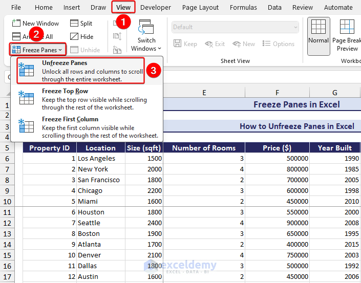
When you’re done with the comparison task that required frozen panes, you might want to unfreeze the panes using the Unfreeze Panes option. Unfreezing panes is the ability to scroll freely through the entire sheet again.
- First, go to the View tab>> click on the Freeze Panes dropdown >> select the Unfreeze Panes option.
Alternatives to Freeze Panes in Excel
If we can not use the Freeze Panes option for any restrictions, we can follow these 3 alternatives to achieve the same goal as Freeze Panes.
1. Using Split Option from the View Tab
You can split your worksheet in 3 different ways. These are splitting horizontal, vertical, and four-way.
Split Horizontally
My spreadsheet has headers that I want to keep visible while scrolling through the data. So, I want to split the panes horizontally. I can use the Split option from the View tab.
- Select an entire row. I selected the 12th row.
- Click on the View tab >> select Split. As a result, the worksheet is split horizontally.
Split Vertically
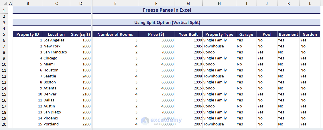
I can split the panes vertically. When you want to see the same dataset side by side, you can use this method.
- Initially, click on the column along which you want to split. I selected the E column.
- Click on the View tab >> Select the Split option shown in the previous method. Now, you have split the worksheet vertically.
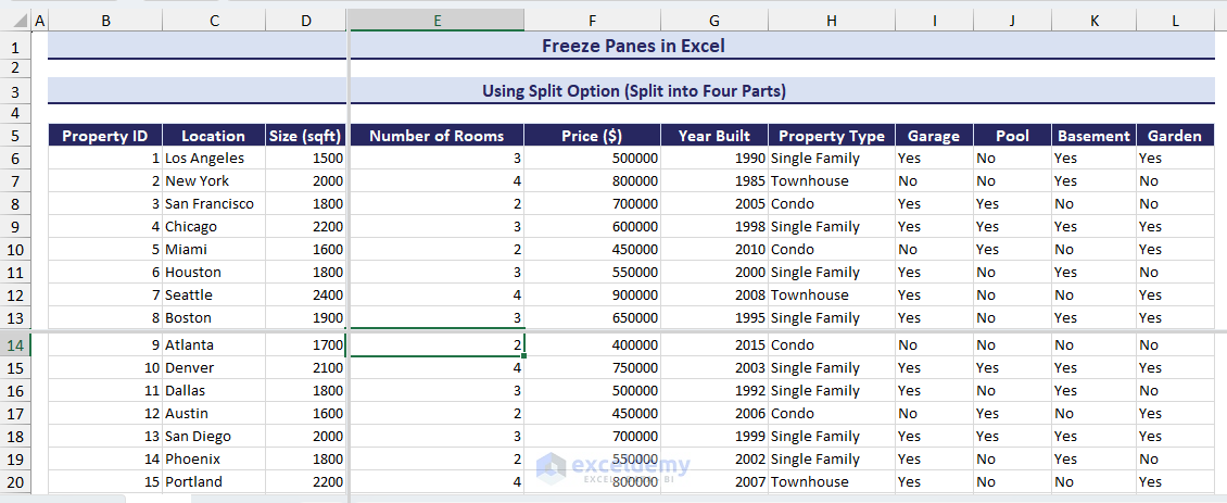
Split into Four Parts
Sometimes you may need to split the worksheet into four parts. It happens when the dataset is very large, and you have to compare lots of information.
- First, click on the cell along which you want to split the sheet into four parts. I selected cell E14.
- Now, select the Split option like the previous methods. Thus, the worksheet is split into four parts. You can scroll each part individually.
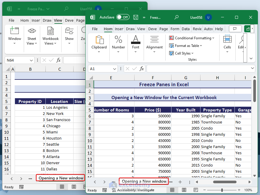
2. Opening a New Window for the Current Workbook
You can open multiple windows in Excel at a time. It is easier to compare multiple Excel sheets opened in each window.
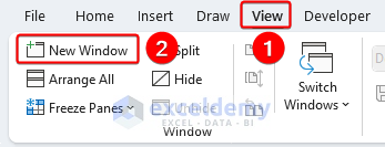
- First, click on the View tab >> You will see the New Window option under the Window group.
- Upon clicking on the New Window option, you see a new window appears.
- Now you can open the same sheets but different columns in these windows to compare data.
3. Inserting Table to Lock the First Row
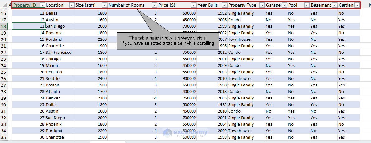
In the Excel table, the top row is visible while scrolling. I use this feature to work as freezing the top row.
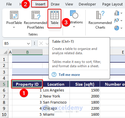
- Click on any cell of the dataset >> go to the Insert tab >> you will notice the Table option.
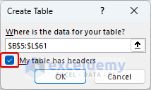
- Select the Table A small selection box will appear. Tick the My table has headers checkbox.
- Click on OK. This will create a table. Now while scrolling, if you select any cell in the table, the table header row will always be visible.
What Are the Reasons That Causing Freeze Panes Not Working in Excel?
- If you have selected or are currently in the Page Layout view, the Freeze Panes option will be greyed out or disabled. So, first change that to Normal view.
- If you have already frozen rows or columns, it will not work. You need to unfreeze them before applying freeze panes to a different area.
- There is a possibility that the worksheet is protected. It prevents you from freezing panes.
- If you are in editing mode, the Freeze Panes option will not be available.
- Sometimes, if you don’t have enough data to require a scroll bar, the freeze panes feature might not work.
Download Practice Workbook
In this article, I have shown how to freeze panes in Excel for different scenarios. It includes freezing the top row, first column, multiple rows or columns, freezing multiple rows and columns together, unfreezing columns, etc. Moreover, VBA code to freeze multiple rows and columns is also described. I hope this article helped you to know about Excel’s Freeze Pane feature in depth. Now, you can use this feature successfully anywhere you need it. If you have any questions regarding this topic, please leave a comment so that we can help.