How to Apply Custom Freeze Panes in Excel (3 Easy Ways)

In this article, we will demonstrate how to use custom freeze panes in Excel. We can easily lock the first row or column from the ‘Freeze Panes’ option directly, but here, we will use the ‘Freeze Panes’ option to lock any rows or columns we want.

Method 1 – Using Freeze Panes Feature to Freeze Custom Rows and Columns

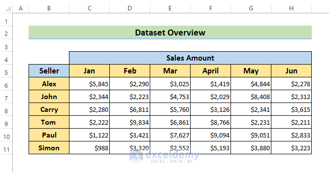
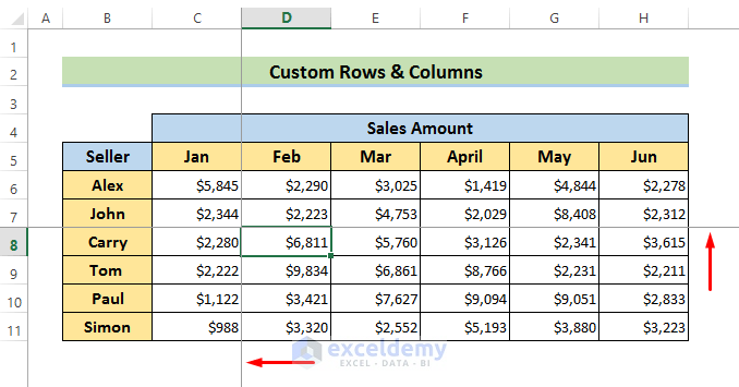
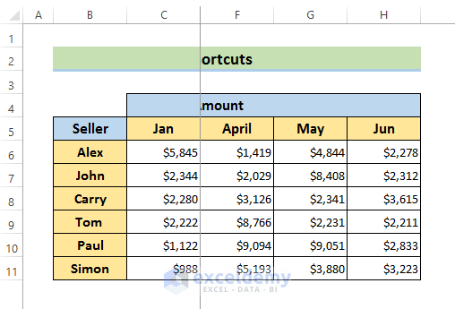
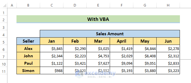
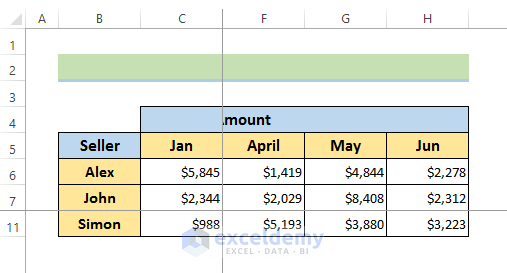
We can freeze rows or columns in our Excel worksheet using the ‘Freeze Panes’ tool. To illustrate how, we will use the following dataset containing the sales amounts of some salesmen for the first six months of a year.

Steps:

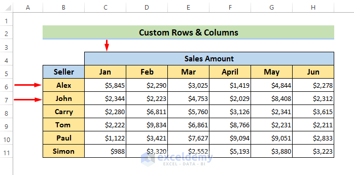
Decide which rows and columns to freeze. Here, we will lock Columns C and B, along with Rows 6 and 7.

To freeze Columns C & B and Rows 6 & 7, select Cell D8.

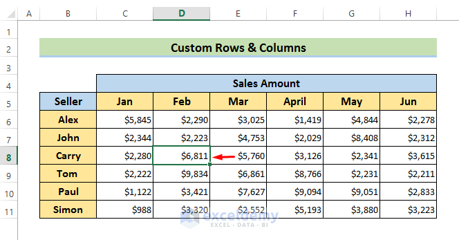
To lock columns and rows simultaneously, select a cell just below the row and just to the right of the column you want to freeze.
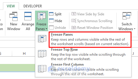
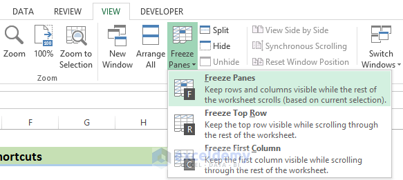
Go to the View tab and select Freeze Panes.

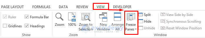
From the drop-down menu that opens, select Freeze Panes.

A horizontal line and a vertical line appear in the worksheet like below.

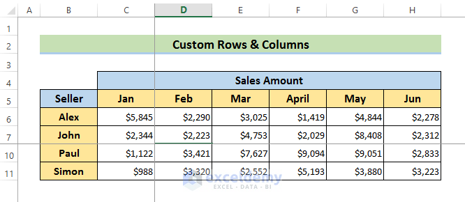
If we scroll down, Row 6 & 7 are locked.

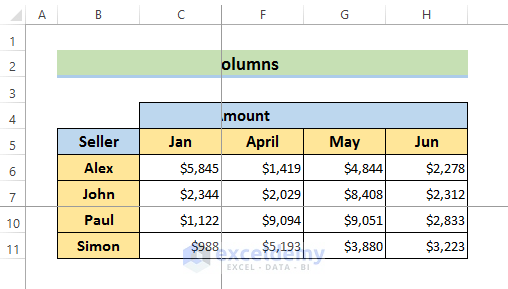
Similarly, if we scroll left to right, Columns C & B are also locked.

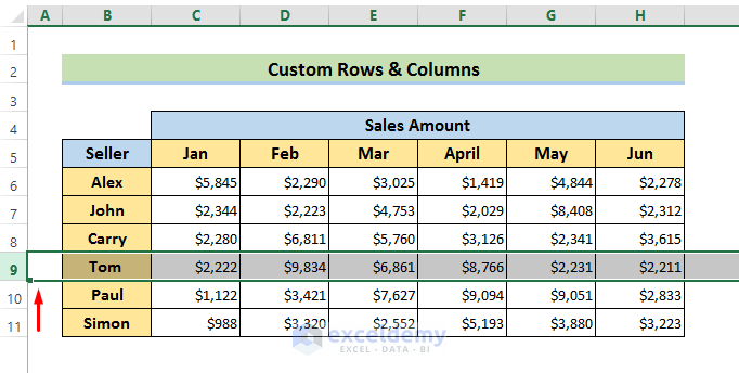
To freeze any specific rows, select the row just below the rows you need to freeze, such as Row 9 here.

Go to the View tab and select Freeze Panes as above.
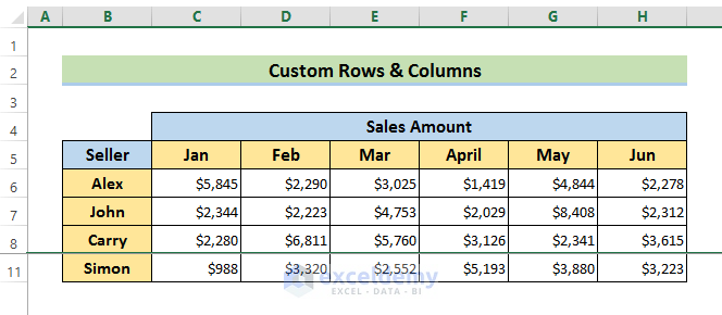
Scroll down.

Rows 6, 7 & 8 are frozen.

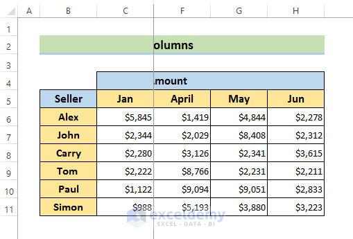
To freeze a column, just select the column next to it.

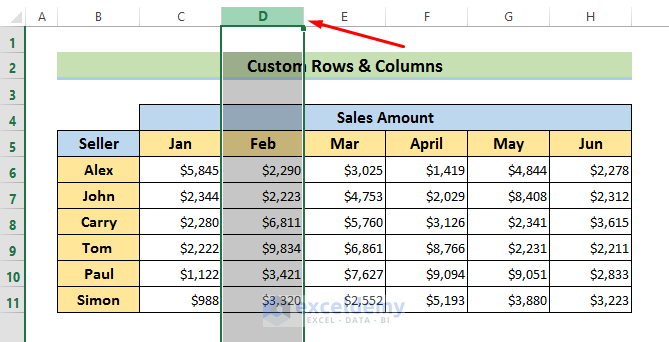
Use the previous steps to return results like below.

Read More: Excel Freeze Panes Not Working

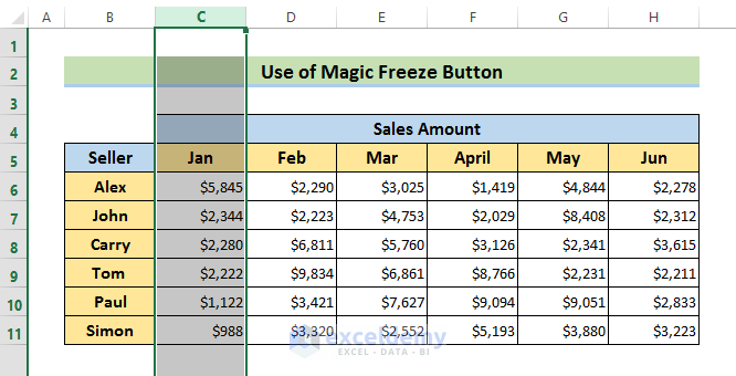
Method 2 – Using the Magic Freeze Button

We can save time and energy freezing any rows or columns with a customized Quick Access Toolbar.

Steps:

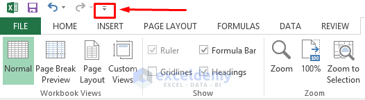
Go to the ‘Customize Quick Access Toolbar’ icon in the upper left corner of the screen.

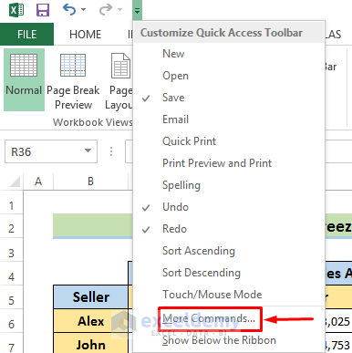
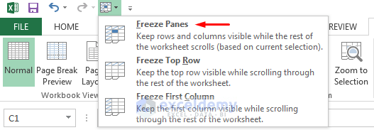
Select ‘More Commands’ from the drop-down menu.

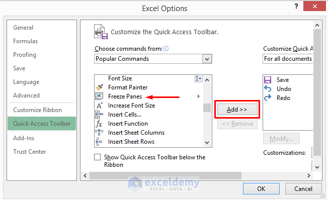
Select ‘Freeze Panes’ from the ‘Choose commands from’.
Click ‘Add’ and then OK to include the button in the toolbar.

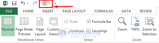
A new icon will appear in the Quick Access Toolbar, the Freeze Panes magic button.

Select Column C to lock Columns A & B.

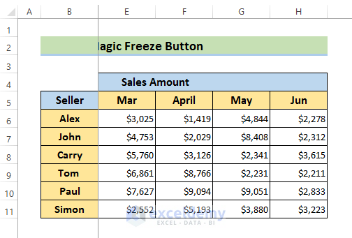
Select the Freeze Panes icon and Freeze Panes from the drop-down menu that opens.

Columns A & B are frozen like below.

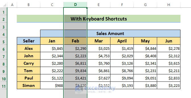
Method 3 – Using Keyboard Shortcuts to Apply Custom Freeze Panes

The keyboard shortcut to freeze rows or columns is Alt + W + F + F.

Steps:

Select the column to the immediate right of the column we want to freeze. We select Column D here because we want to freeze Columns A, B & C.

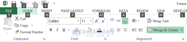
Press the Alt key to reveal a ribbon like below.

Press W, which will open the View tab.

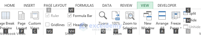
Press F. This will open the drop-down menu of Freeze Panes.

Again press F to freeze the desired columns.

Freeze Rows & Columns with VBA in Excel

Excel VBA also gives us the opportunity to custom freeze rows, columns, and cells in our dataset.

Steps:

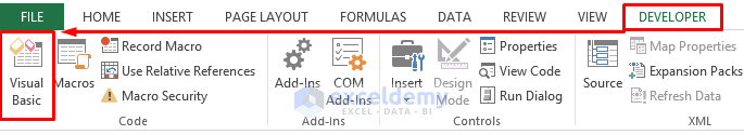
Go to the Developer tab and select Visual Basic.

Go to Insert and select Module.
Enter the following code in the Module and Save it:

Sub Lock_Row()
   ActiveWindow.FreezePanes = False
   Rows("8:8").Select
   ActiveWindow.FreezePanes = True
End Sub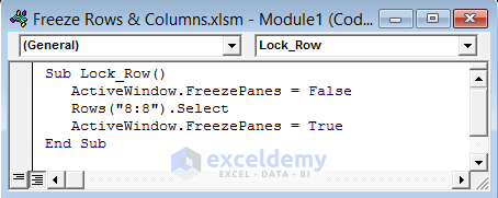

Here, we want to lock the rows above Row 8, so we put “8:8” in the code.

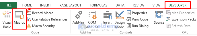
Go to Macros on the Developer tab.

Select Run from the Macro window that opens.

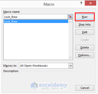
Run the code.

The rows above Row 8 are frozen.

To freeze a specific column, enter the code below:

Sub Lock_Column()
   ActiveWindow.FreezePanes = False
   Columns("C:C").Select
   ActiveWindow.FreezePanes = True
End Sub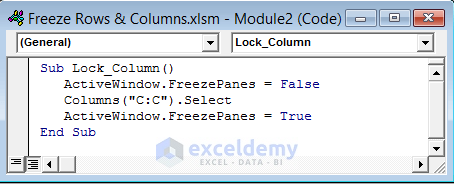

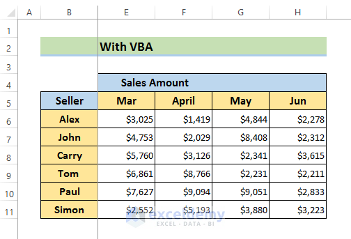
After running the code, Columns A & B are frozen.

To freeze rows and columns simultaneously, enter the code below:

Sub Lock_Cell()
   ActiveWindow.FreezePanes = False
   Range("D8").Select
   ActiveWindow.FreezePanes = True
End Sub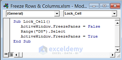

After running the code, Columns A, B & C and the rows above Row 8 will be frozen.

Things To Remember

You cannot lock columns or rows in the middle of your worksheet. You can only freeze rows above the selected row and columns on the left side of the worksheet.
The Freeze Panes command will not work when you are in editing mode. To cancel edit mode, press the Esc key.

Download Practice Book

Custom Freeze Panes.xlsm

<< Go Back to Freeze Panes | Learn Excel

Get FREE Advanced Excel Exercises with Solutions!