How to Unfreeze Rows and Columns in Excel (with Quick Steps)

We frequently work with Excel datasets. For example, when scrolling through a vast dataset, you may need to freeze some rows or columns to keep them visible. However, unfreezing rows or columns in Excel is a simple operation. In this post, we’ll show you how to unfreeze rows and columns in Excel.

How to Unfreeze Rows and Columns in Excel: Quick Steps

You can easily unfreeze rows and columns in Excel.

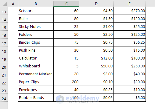
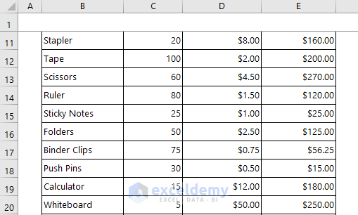
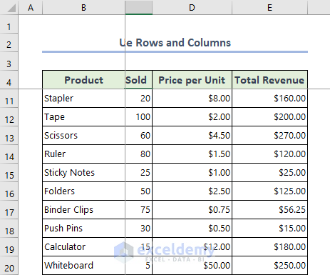
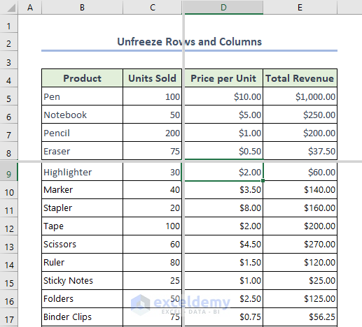
Here we have a dataset that contains some stationary products, their unit price, the number of items sold, and the total revenue.

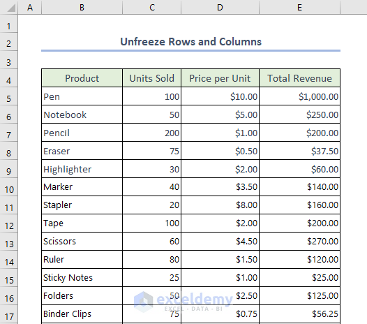
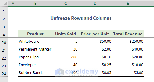
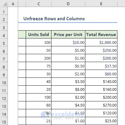
Here the dataset has frozen rows and columns.

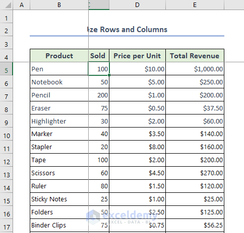
In the above image, you can see that the 1st two columns are frozen. So, when you move the worksheet horizontally, the products column is fixed and visible constantly.

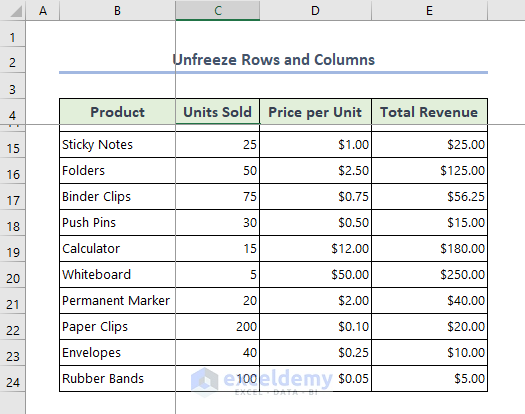
Again for the rows, in this Excel sheet, the rows are fixed up to the title row. So if you scroll vertically, the first four rows will be fixed.

Now we will unfreeze these rows and columns. In the next part, we will show you the steps of how to unfreeze rows and columns in an Excel sheet.

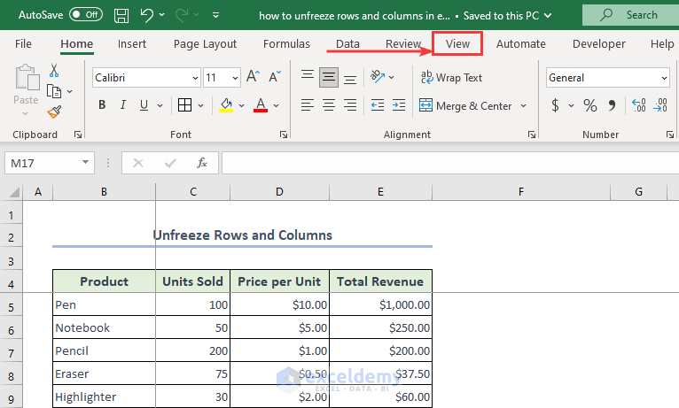
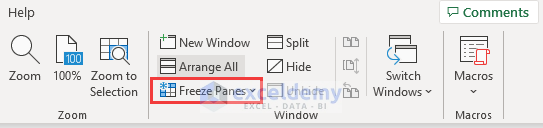
Step 1: Click on the View Tab

First, we will have to click on the View tab from the ribbon.

Step 2: Select ‘Freeze Panes’ from Window Section

Next, after clicking the View tab, you can see some groups.
Find the Freeze Panes command from the Window group and click on it.

Step 3: Choose ‘Unfreeze Panes’ from Drop-Down Menu

After that, click on the dropdown menu, and you will see a few options.
If the Excel sheet has frozen rows/columns, then it will show Unfreeze Panes on the first option of the dropdown menu.
Select the option.

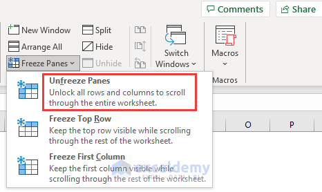
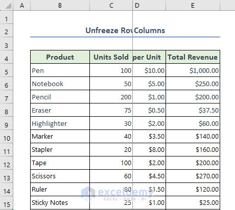
Finally, the rows and columns will be unfrozen.

How to Freeze Rows and Columns in Excel

We sometimes need to freeze rows and columns in extensive datasheets. Freezing rows and columns is a very easy task. But we have to follow a few steps to do that. Below we will show you how to freeze any row or column, also rows and columns at the same time.

1. Freeze Rows in Excel

First, if you want to freeze the first row of the sheet, you can go to the View tab.
Next, click on Freeze Panes and select Freeze Top Row from the dropdown menu.

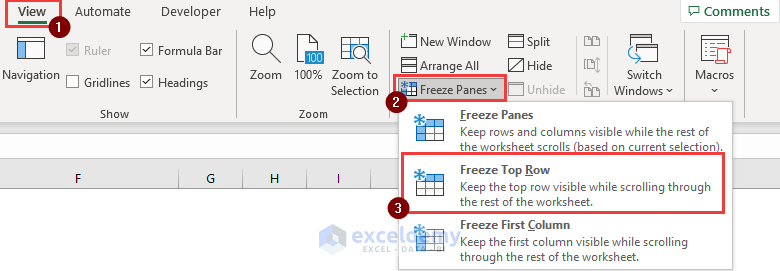
Then, you will see only the top row will be frozen.

If you want to freeze multiple columns, select the row just after the last row you want to freeze.
After that, go to View >> Freeze Panes >> Freeze Panes (drop-down menu).
And you will see the rows above selection will be frozen.

2. Freeze Columns in Excel

You can also freeze columns in Excel. To freeze the first column, go to View >> Freeze Panes >> Freeze First Column.

You can also freeze multiple columns in Excel.
First, select the column right to the last column you want to freeze.
Then, go to View >> Freeze Panes >> Freeze Panes.
Finally, multiple columns will be frozen.

3. Freeze Rows and Columns at the Same Time

You can also freeze rows and columns at the same time in Excel. Follow the next steps to be able to do that.

In the beginning, you need to select the cell that is right after the rows and columns you want to freeze.
Suppose you want to freeze up to the 4th row and B
Then, you have to select cell C5.
Afterward, go to View >> Freeze Panes >> Freeze Panes.
Next, you will see the top four rows and two columns are frozen simultaneously.

Freeze Vs Lock Command in Excel

If you want to keep any row or column always visible in the sheet still when you are scrolling, you need to apply the Freeze feature.

The Lock feature in Excel is different from the Freeze feature. The Lock feature locks the contents of a cell. It prevents making any changes to a locked cell, range, list, formulas, etc.

So, freeze and lock are not the same features.

Other View Options in Excel

There are other features in the View tab of Excel to work efficiently with worksheets. In large datasheets, these options help in many ways, such as opening a new window or splitting a worksheet.

Open New Window in Excel

You can easily open the current workbook in a new Excel window. This feature helps to compare data in large datasheets. Here are the steps on how to do that.

First, go to the View tab and click on the New Window

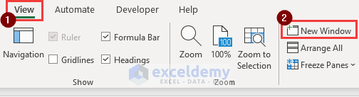
Next, a new window will appear on the screen.

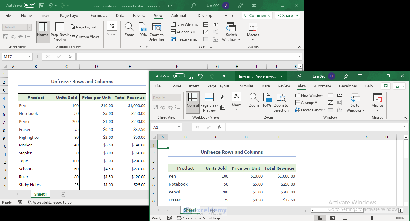
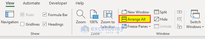
If you open many windows, you can organize them using the Arrange All option, just below the New Window

Splitting a Worksheet

The Split feature in the View tab is a fantastic feature that allows scrolling different parts of a worksheet. You can split the worksheet into small panes and scroll data in that portion independently.

First, go to the View tab and select the Split

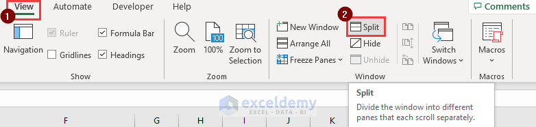
It will split the dataset into smaller panes. Then, you can scroll through the panes individually.

You can easily remove the Split and go back to the previous version again by clicking on the Split button again,

Things to Remember

Only rows and/or columns that are visible on the screen can be frozen. To freeze rows or columns that are not currently visible, you must first scroll to them.
You can quickly freeze or unfreeze rows and columns by clicking and dragging the line between the row or column headers. Dragging it down or to the right will cause that row or column to be frozen. Unfreezing it is as simple as dragging it back up or to the left.

Download Practice Workbook

Unfreeze Rows And Columns.xlsx

Conclusion

In this article, we showed how to unfreeze rows and columns in Excel. We sincerely hope you enjoyed and learned a lot from this article. If you have any questions, comments, or recommendations, kindly leave them in the comment section below. Stay with us and keep Excelling!